Section 4 :: Carrying Capacity to Competition

Flow Diagram for the Logistic Equation

Get out some scratch paper and sharpen that pencil. There aren’t any code blocks in this Section, but it is sooo important that you practice drawing/interpreting the diagrams and solving the problems on paper. Absorbing this material by staring at it is not an effective way to approach it

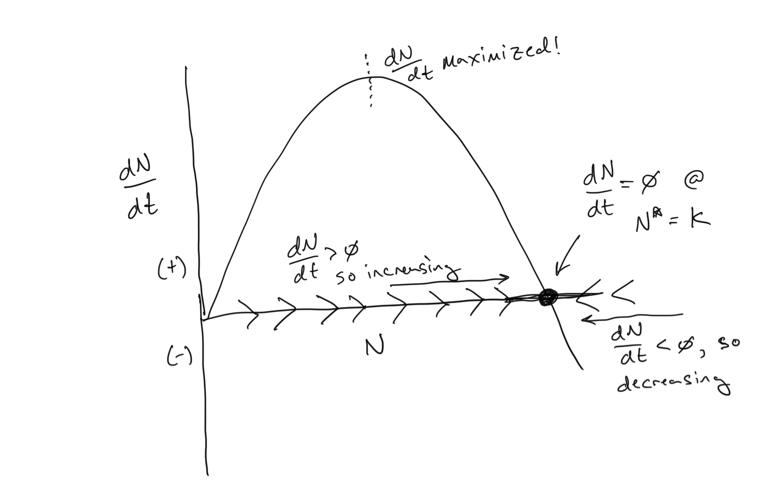
Our population growth equation that incorporates density-dependent per-capita birth and death rates is known as the Logistic Equation. You can see above how it has a sigmoidal shape… population growth begins exponentially but then tapers off as it reaches the carrying capacity $K$. And we have used the per-capita birth and death rates to anticipate the dynamics using the flow concept. Below we see that we can use the flow concept in a different way… to examine $dN/dt$ as a function of $N$.

$dN/dt$ as a function of population size $N$ for the *logistic equation*. Similar to looking at how per-capita birth and death rates change with population size, we can use the concept of *flow* to anticipate the dynamics of the system. Flow goes from left to right along the *x-axis* (increasing population size $N$) when $dN/dt > 0$ and it goes from right to left along the *x-axis* (decreasing population size $N$) when $dN/dt < 0$.

Discussion

Where is the carrying capacity $K$?

There are two values of $N$ where $dN/dt = 0$. What are they?

Where is $dN/dt$ maximized on the plot above? Can you guess the value of $N$ corresponding to where $dN/dt$ is maximized? What is special about this point in terms of how the population changes over time?

Bonus round: Can you analyitically solve for the point at where $dN/dt$ is maximized in terms of $N$? Hint: to do this you would need to take the derivative of something…

Interpret the following diagrams

Make sure that you understand what all of the relationships mean and can elucidate expectations for what the population will do over time! I recommend that you either a) print out the below figure, or better yet b) transcribe it yourself onto a sheet of paper so that you can draw and label the various elements to help you interpret what is going on.

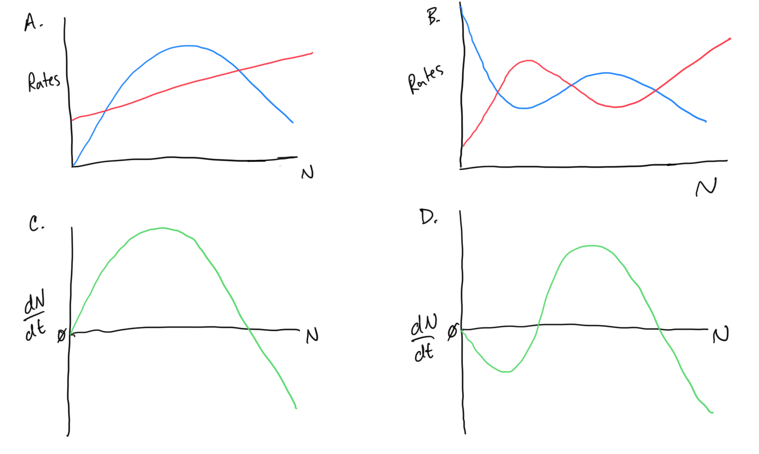
Interpret these diagrams! As before the BLUE line is the per-capita birth rate, and the RED line is the per-capita death rate.

Discussion

For each of the above diagrams… where are the steady states? What is the flow above or below the steady states? What will happen to the population given that it starts at various places along the x-axis?

In which diagrams can you say something about how quickly the population changes over time? Where is population change fast, where is it slow?

In which diagrams is there an Allee effect (if any)? Why?

Including the basics effects of competition!

Consider a population that is growing in accordance with the Logistic Equation (remember that we are in continuous time now) of the form

\[\begin{equation} \frac{\rm d}{\rm dt}N_1 = r_1 N_1\left(1 - \frac{\color{red}{N_1}}{K_1}\right). \end{equation}\]

We must now recognize that we are (and have been) incorporating the effects of competition for quite some time, as the Logistic Equation illustrates. Early in its growth (when the environment is empty and has plenty of resources to go around) the population $N_1$ grows near-exponentially. As the population reaches carrying capacity, $N_1\rightarrow K_1$ and the growth drops to zero as the population reaches the steady state $N_1^*=K_1$. These key behaviors of Logistic Growth can be observed by focusing on the numerator in the Logistic Equation, highlighted in $\color{red}{\rm red}$. If $N_1$ is close to zero, the numerator is close to zero, meaning $dN_1/dt$ approximates $r_1 N_1$. If $N_1$ is close to $K_1$, the numerator is close to one, meaning $dN/dt$ is close to zero. The numerator is encoding the negative effects of intraspecific competition on the growth of the population. As more individuals are added to the population, the numerator increases, slowing down growth.

Including both Intraspecific and Interspecific competition

We will now consider a second species, with population density $N_2$. Initially we can assume that $N_2$ changes over time… so it is a constant. The population of the competitor $N_2$ will stay the same even as $N_1$ changes over time (we will relax this assumption in the next section). The population of $N_2$ has a negative effect on the population of $N_1$, very similar to how a larger population $N_1$ is expected to limit resources, slowing down ${\rm d}N_1/{\rm dt}$ as codified in the Logistic Equation.

Let’s state some assumptions… if individuals in population $N_2$ are doing the same things (for example using the same resources) as individuals in population $N$, we expect them to have the same effect on slowing down the growth of population $N_1$. If the individuals in population $N_2$ are doing very different things (for example using mostly different resources) as individuals in population $N_1$, we expect them to have less of an effect on the growth of population $N_1$.

Let’s introduce a parameter $\alpha$ that captures this relationship. If $\alpha=1$ we will say that the competitors $N_2$ are using the same resources as the population $N$. If $\alpha < 1$, we will say that the competitors are using very different resources. So now let’s introduce this into the Logistic Equation:

\[\begin{equation} \frac{\rm d}{\rm dt}N_1 = r_1 N_1\left( 1 - \frac{\color{red}{N_1 + \alpha N_2}}{K_1}\right) \end{equation}\]

Note that now there are multiple factors to consider in terms of their influence on the numerator.

Discussion

What factors slow down growth when they change in which direction?

What does it mean if $\alpha = 1$ or if $\alpha < 1$ (assume that $\alpha$ remains strictly positive). What does it mean if the size of the competitors population $N_2$ is large or small for a given value of $\alpha$? In other words, how do these variations impact ${\rm d}N_1/{\rm dt}$?

Solve for ${\rm d}N_1/{\rm dt} = 0$. How does introducing a competitor alter our expectations from Logistic Growth?

Consider what values of $\alpha > 1$ might mean in terms of the effect that individuals in $N_2$ have on the growth of population $N_1$.

The Lotka-Volterra Competition model

We will now consider the dynamic feedback that one competing species has on the other competing species and vice versa. Let us use the following illustration to guide our setup.

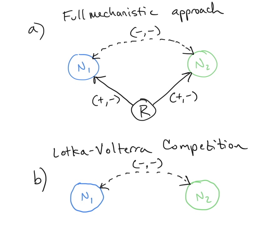
a) A full mechanistic description of two species competing for a common resource $R$. b) The simpler setup that is captured in the Lotka-Volterra Competition equations, where the negative effects that each species has on the other is included, however the explicit consumption for a shared resources is not.

The Lotka-Volterra Competition framework examines the population growth of competing species $N_1$ and $N_2$. Both the negative effects of intraspecific as well as interspecific competition are now included for both… look at that numerator! The interaction terms included are exactly those we examine above, but where the populations of $N_1$ and $N_2$ both change over time. The LV Competition equations are thus written

\[\begin{align} \color{blue}{\frac{\rm d}{\rm dt}N_1} &= \color{blue}{r_1 N_1\left( 1 - \frac{N_1 + \alpha N_2}{K_1}\right)} \\ \\ \color{green}{\frac{\rm d}{\rm dt}N_2} &= \color{green}{r_2 N_2\left( 1 - \frac{N_2 + \beta N_1}{K_2}\right)} \end{align}\]

We call this system a 2-dimensional system because we are tracking changes in two densities: the population density of $N_1$ and the population density of $N_2$. There are 3 parameters for each population:

Variables:
$N_1$: Population density of species 1
$N_2$: Population density of species 2
Parameters
$r_1,~r_2$: Intrinsic growth rates of species 1 and 2, respectively
$K_1,~K_2$: Carrying capacities of species 1 and 2, respectively
$\alpha$: The per-capita effect of species 2 on the growth of species 1
$\beta$: The per-capita effect of species 1 on the growth of species 2

One thing that we want to ingrain into our consciousnesses is to immediately examine the steady state solutions when we see equations like these. Where does the population come to rest over a long enough time? Where is the steady state? Let’s first take a look at a single dimension of this (now) 2-dimensional problem. Let’s set $dN_1/dt = 0$ and solve for $N_1^*$. Remember we use the ${}^*$ to denote the value of the population at steady state, which is just a special population size that carries with it dynamical importance.

\[\begin{align} &\color{blue}{\frac{\rm d}{\rm dt}N_1} = 0,~{\rm so} \\ \\ &\color{blue}{r_1 N_1^*\left( 1 - \frac{N_1^* + \alpha N_2}{K_1}\right)} = 0, \\ \\ &{\rm giving~two~solutions.~ Either~}\color{blue}{N_1^*} = 0,~{\rm or} \\ \\ &\color{blue}{\left( 1 - \frac{N_1^* + \alpha N_2}{K_1}\right)} = 0 \\ \\ &{\rm which~simplifies~to~}\color{blue}{N_1^*}=\color{blue}{K_1 - \alpha N_2} \end{align}\]

Is this the same or different than what we observed before we added the dynamics for $N_2$? Note that we did not use the ${}^*$ notation for $N_2$ because we did not stipulate that $dN_2/dt = 0$.

What does this equation simplify to if $N_2$ is driven to extinction? Let’s draw a new graph, where we have the density of population $N_1$ on the x-axis and the density of $N_2$ (which we are now assuming to be zero given it is extinct). We compute the steady state of this system in the following way:

\[\begin{align} N_1^* &= K_1 - \alpha N_2 \\ \\ N_1^* &= K_1 - \alpha \cdot 0 = K_1 \end{align}\]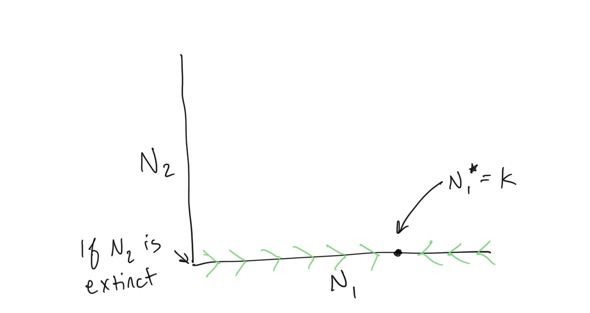

Establishing where the population $$N_1$$ is growing or declining when population $$N_2$$ has gone extinct.

Now we want to establish the flow along the x-axis, but we do not currently have a nice set of birth and death relationships to show us when the population is growing or shrinking. Instead, we will ask the equation itself! For example, we will reduce the inequality $dN_1/dt < 0$ to find under what conditions the population is declining, and likewise will reduce the inequality $dN_1/dt > 0$ to find under what conditions the population is increasing.

Where is the population $N_1$ declining???

\[\begin{align} &\color{blue}{\frac{\rm d}{\rm dt}N_1} < 0 \\ \\ &\color{blue}{r_1 N_1\left( 1 - \frac{N_1 + \alpha N_2}{K_1}\right)} < 0, \\ \\ &{\rm giving~two~solutions.~ Either~}\color{blue}{r_1 N_1} < 0,~{\rm or} \\ \\ &\color{blue}{ 1 - \frac{N_1 + \alpha N_2}{K_1}} < 0. \\ \\ &{\rm Given~that~we~are~assuming~}r_1>0~{\rm and~}N_1>0,{\rm ~we~will~consider~only~the~second~condition} \\ \\ &\color{blue}{1 - \frac{N_1 + \alpha N_2}{K_1}} < 0 \\ \\ &\color{blue}{1} < \color{blue}{\frac{N_1 + \alpha N_2}{K_1}} \\ \\ &\color{blue}{K_1} < \color{blue}{N_1 + \alpha N_2} \\ \\ &{\rm and~IF~}N_2 = 0,~{\rm then} \\ \\ &\color{blue}{K_1} < \color{blue}{N_1},~{\rm or~in~other~words} \\ \\ &\color{blue}{N_1} > \color{blue}{K_1} \end{align}\]

So if we carefully keep track of our inequalities (if you need a reminder of the inquality rules when doing algebra, check out this resource), we find that the condition $dN_1/dt < 0$ (population decline) is true when $N_1 > K_1$. So in the graph above we draw our flow from right to left above the point $K_1$.

Discussion

Solve for the opposite condition $dN_1/dt > 0$ and ensure this algebraic result matches where you think the left-to-right flow should occur in the graph above.

Now solve for the same conditions but without our assumption of the extinction of $N_2$.

The answer to question 2 is a line on the $N_2$ vs. $N_1$ graph. What does this line represent?

What are the x- and y-intercepts of this line?

Establishing where the population $N_1$ is growing or declining with respect to any size of the $N_2$ population. The line is labeled the $N_1$ isocline because it is defined by the condition $dN_1/dt = 0$. In other words, at any point along this line, the population $N_1$ *will be at steady state*.

Finding the FLOW in 2-Dimensional Space

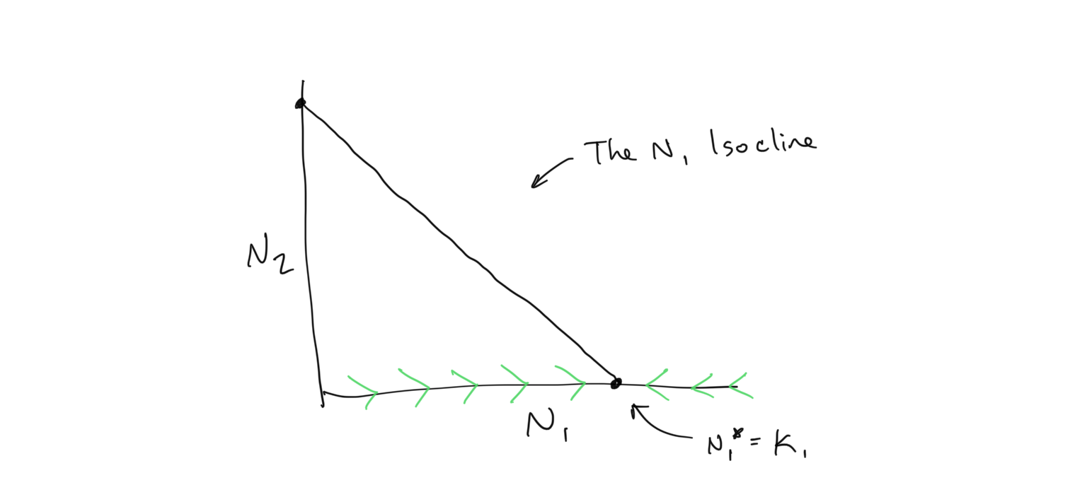
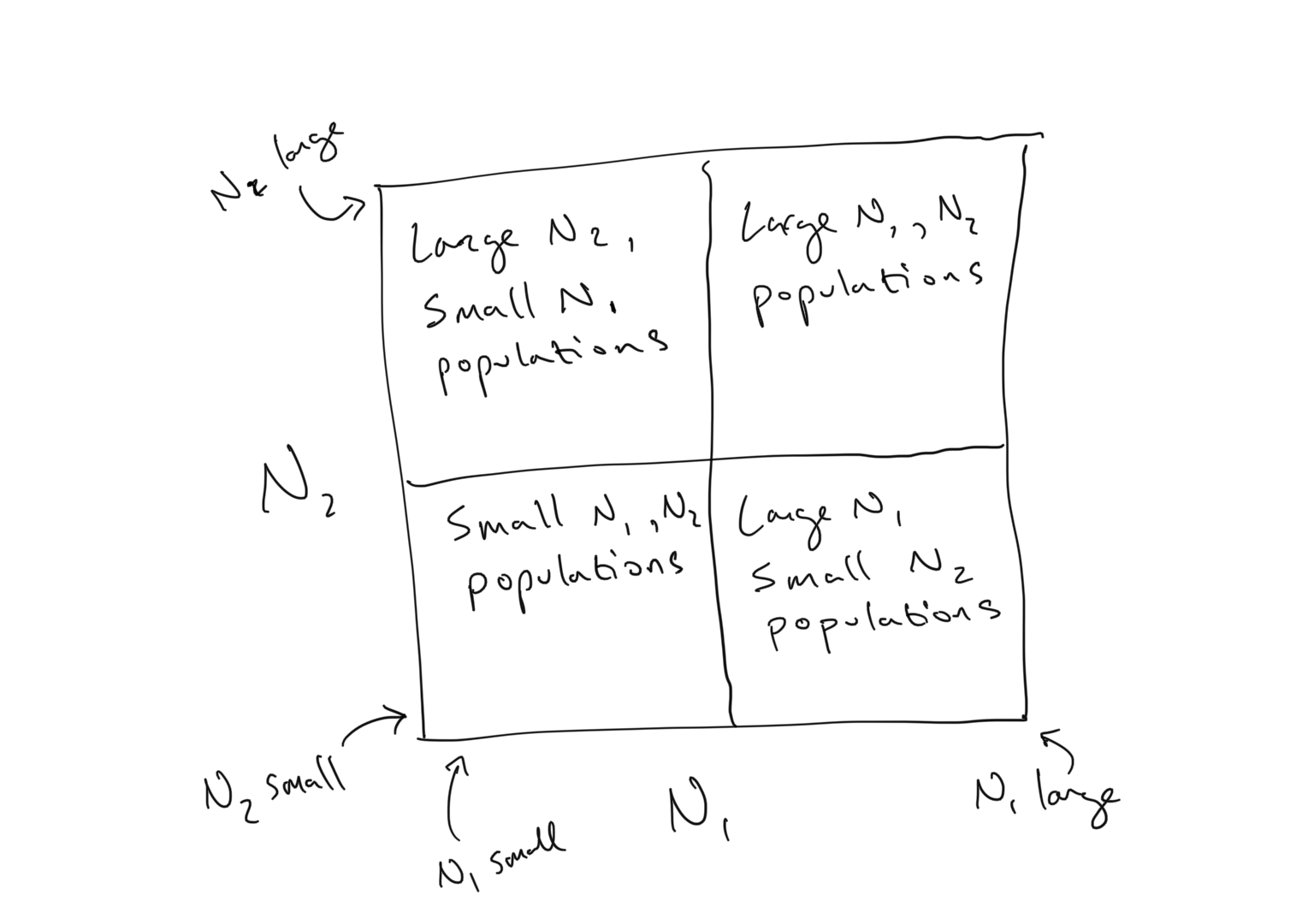
As we observe above, an isocline is a line along which the growth of a population is zero… i.e. a line that defines the steady state of a population. The 2-dimensional $N_2$ vs. $N_1$ space represented in the figures above displays any combination of population values for the species in the competition system, which we can visualize in terms of quadrants

Quadrants in 2-dimensional $N_2$ vs. $N_1$ space describe different combinations of population size for the competition system.

The $N_1$ isocline within this space represents the region where $dN_1/dt = 0$. This line is a dimensional extension of the steady state existing as a single point when we just had 1 population to consider (i.e. 1 dimension)… In 1-dimension the steady state is a point along the $N_1$ line… in 2-dimensions the steady state is a line cutting across the $N_2$ vs. $N_1$ plane.

We find the isocline by setting $dN_1/dt = 0$
We reconstruct the flow by reducing the inequalities… where does the population $N_1$ grow such that $dN_1/dt > 0$? Where does the population $N_1$ decline, such that $dN_1/dt < 0$?

By following the algebraic steps for dealing with these inequalities as presented above, we find

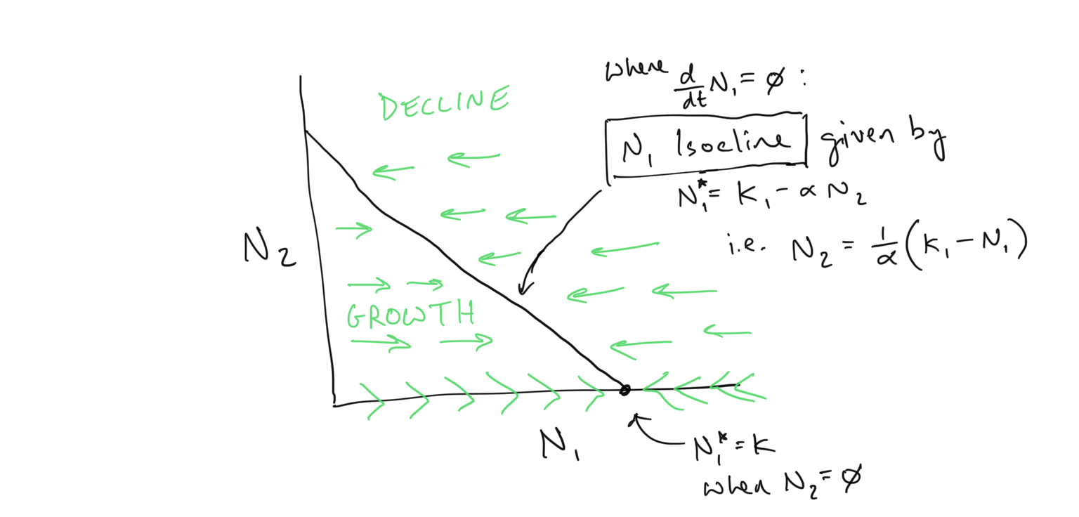
The $N_1$ isocline is given by $N_1^* = K_1-\alpha N_2$
Growth of $N_1$ ($\rightarrow$) occurs when $N_1 < K_1 - \alpha N_2$
Decline of $N_1$ ($\leftarrow$) occurs when $N_1 > K_1 - \alpha N_2$

We can draw this flow within the coordinate space of $N_2$ vs. $N_1$ as

The isocline drawn on the 2-D $N_2$ vs. $N_1$ space, as well as the FLOW now visualized along a plane instead of a line... We find this flow by reducing $dN_1/dt < 0 $ and $dN_1/dt > 0 $. We find that the isocline defines the cross-over from *growth* to *decline*.

What about $N_2$?

You might be wondering *what about $N_2$? As you might guess, we now will perform the same exercise:

Find the $N_2$ isocline by solving for $dN_2/dt=0$
Determine the flow on either side of the isocline by reducing the inequalities $dN_2/dt < 0$ (where $N_2$ declines) and $dN_2/dt > 0$ (where $N_2$ grows)

Opposite of the flow for $N_1$, the flow of $N_2$ as we have drawn it above will be along the vertical axis, or y-axis, because this is the axis corresponding to the population size of $N_2$. Here is what we obtain

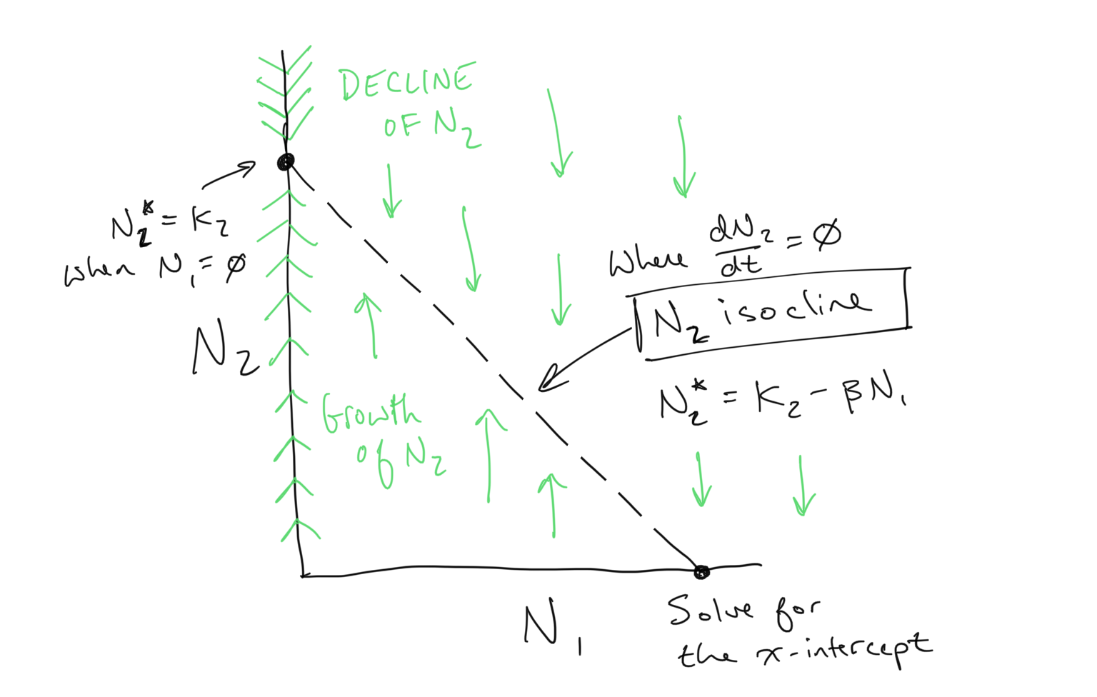
The $N_2$ isocline, depicting the region where $dN_2/dt=0$, and the flow of population $N_2$, in terms of growth or decline, on either side. The flow is along the *y-axis* because this is the axis denoting the size of population $$N_2$$.

Discussion

Derive the equation for the $N_2$ isocline

Derive the y-intercept and x-intercepts for the $N_2$ isocline

Compare the x,y-intercepts and slopes for the $N_1$ and the $N_2$ axes. What parameters determine the intercepts and slopes of each? Understanding this will be key for piecing together the dynamics of this system.

Putting it all together

We have derived the $N_1$ isocline and we have derived the $N_2$ isocline. We have also determined the flow along the x- and y-axes on either side of each isocline. This is all of the information we need to determine the dynamics of the Lotka-Volterra Competition model. We just need to put it together.

We will examine the dynamics for the full system by plotting both isoclines and both flow regimes in the same figure. Depending on the intercepts and slopes for the $N_1$ and $N_2$ isoclines, different isocline arrangements are possible, and it is these arrangements that determine the dynamics. Observe the example below

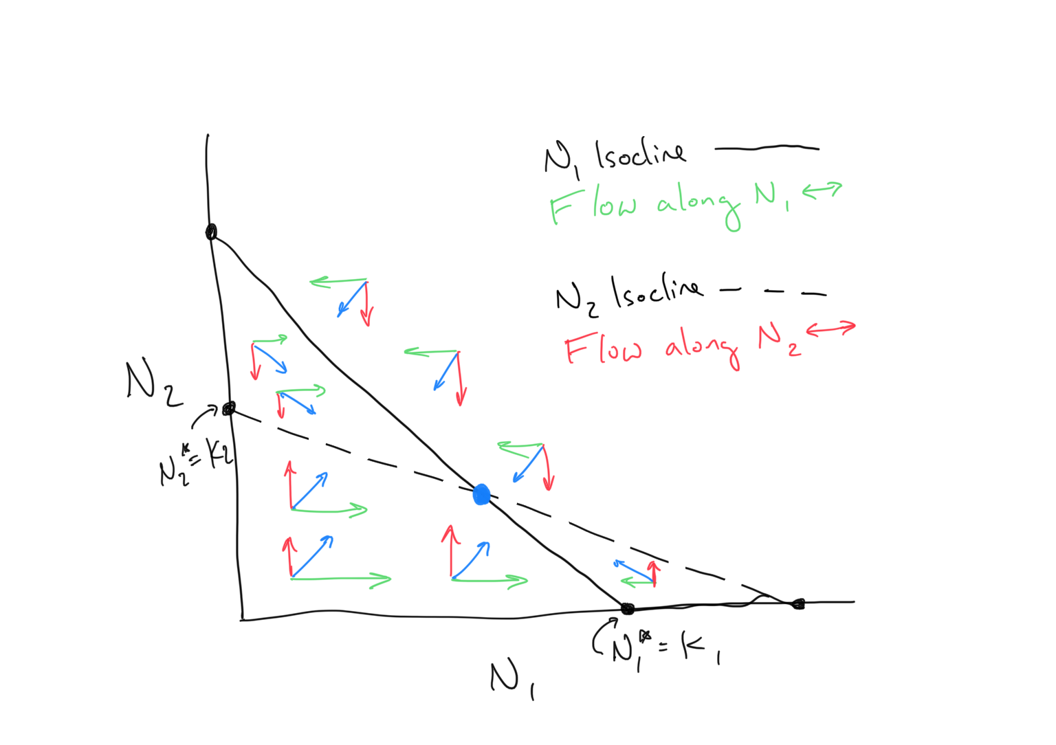
The $N_1$ (solid black line) and $N_2$ (dashed black line) isoclines, with respective flows along the $N_1$ (green) and $N_2$ (red) axes. The green and red flows show the relative influence of each isocline on the trajectory of the dynamic system (i.e. how $N_1$ and $N_2$ change over time). The blue arrow shows the composite directional flow.

Discussion

Judging from the figure above, what do we expect to happen to the populations of $N_1$ and $N_2$?

What does the blue point represent?

There are three additional possible unique arrangements of the $N_1$ and $N_2$ isoclines depending on the relative placements of the x- and y-intercepts of both (for a total of four). Draw them and sketch out the 2-dimensional flow. What is expected to happen in each of these potential systems? How does the outcome depend on the differences in x- and y-intercepts of the $N_1$ and $N_2$ isoclines?

Try solving for the point where the $N_1$ and $N_2$ isoclines intersect. How would you go about doing this?

Fundamentals of Ecology

Section 4 :: Carrying Capacity to Competition

Flow Diagram for the Logistic Equation

Discussion

Interpret the following diagrams

Discussion

Including the basics effects of competition!

Including both Intraspecific and Interspecific competition

Discussion

The Lotka-Volterra Competition model

Discussion

Finding the FLOW in 2-Dimensional Space

What about \(N_2\)?

Discussion

Putting it all together

Discussion