< Back to Course Page

Part I: Changes in population size over time

Over the course of the last two sections, we have focused our discussion on fitness. How do individual behaviors influence its success in an evolutionary context. But what does success mean? In the terms we have discussed, success is a combination of being able to survive long enough to pass down your genetic material into the next generation, and to ensure that the next generation has what they need to survive themselves. And as we have learned, organisms do this in a variety of ways… they can invest a lot of energy into a few offspring, or they can invest a little energy into a lot of offspring. They can scatter their reproductive events over the course of their lives, or they can wait until the end of their lives to invest in reproduction.

Now let’s take this a step further, and examine how these different strategies influence not an individual, but a collective of individuals, which we call a population. A population is a collection of individuals that interact and reproduce with each other more-so than they might do with other nearby populations. We will eventually discuss metapopulations, where multiple populations are linked together by migration, but for now we will focus our efforts on a single population of a single species.

How do populations change through time? Without the complexities of immigration and emigration, we simply note that populations increase by reproduction (+ Births) and decrease by mortality (- Deaths). So we can write

where B is the total number of births that occur within the time-step \((t+1) - t\) and D is the total number of deaths in that same timestep. As we will explore, the size of the timestep matters. Take 1000 humans… if our timestep is one hour, very few (likley zero) of those individuals will have reproduced or died within that span. If our timestep is one year, it is more likely that some will have given birth, and some will have died. We can generalize the size of the timestep by \(\Delta t\) to not that in some temporal window, births and deaths occur:

This means something slightly different. We are saying that \(B\) and \(D\) represent the total births and total deaths per unit time. So if \(B\) and \(D\) represent total births and total deaths per day, then the size of our temporal window \(\Delta t\) will increase or decrease the total number of births and deaths with respect to the size of the window. If \(\Delta t\) is 30 days, then the total number of births and deaths represent those expected within a month given the daily rates of \(B\) and \(D\). The second line is simply an algebraic manipulation of the first line, showing that within the temporal window \(\Delta t\) the change in that population over that time is equal to the total births minus total deaths.

Now the question is: should we always expect the same number of births and deaths for a given time window regardless of population size? I hope you say no, because that’s the correct answer. Imagine our current population is 10… or imagine it is 10000000. We would expect a different total number of births and deaths, and we would expect this to change as a function of the population size. In this way we can describe the total number of births and deaths as being density-dependent. A simple assumption would be that births and deaths increase linearly with the size of the population. So \(B = bN(t)\) and \(D = dN(t)\). Notice that these are both straight lines with a y-intercept of zero (makes sense… if there are no individuals in the population there are no births or deaths!). Here, \(b\) is the per capita birth rate, and \(d\) is the per-capita death rate. We can then rewrite

where we have defined a new parameter \(r_d = b-d\), which is the average per-capita growth rate of the population. The subscript \({}_d\) reminds us that this is a growth rate specifically for populations that change over discrete rather than continuous intervals. Notice we have also divided both sides by \(\Delta t\), which will help with the next step. Before we move on, let’s examine the current equation for population growth

    discrete.growth = function(N0,tmax,Deltat,b,d) {
        pop = numeric(tmax)
        pop[1] = N0
        for (t in 2:(tmax)) {
            N = pop[t-1]
            NewN = N + Deltat*(b-d)*N
            pop[t] = NewN
        }
        plot(pop,xlab='Time Steps',ylab='Population Size',type='b',pch=16)
    }
    discrete.growth(N0 = 5,tmax = 20, Deltat = 1, b = 0.8, d = 0.7)

Discussion

1. Experiment with the above parameter values. What happens when you change \(b\) to be greater, less-than, or equal to \(d\)? Describe in words what is happening in each scenario.
2. Compare results for small versus large time windows \(\Delta t\) Deltat
3. What is the shape of the population over time when we expand the amount of time over which we observe the population? e.g. try tmax = 100
4. Given \(\Delta t = 1\), what is the proportional change in population size? How would you calculate this? Hint: you don’t need to the code black to do this… Look to the last equation before the code block.

Discrete to Continuous time

As we will (or have) discuss(ed) in class, if we make the time window infinitesimally small (i.e. \(\Delta t \rightarrow 0\)), we can write

A few things to note here… first is that the right-hand-side (RHS) of the equation looks a lot like the discrete time version. However, we now are using \(r\) instead of \(r_d\) to denote the population growth rate. This is because our interpretation of these parameters is a bit different. Here \(r\) is the instantaneous rate of growth of the population. To put this equation into words, we would say: the change in the population over time is equal to rN, where r is the instantaneous rate of growth and N is the size of the population.

You can use CALCULUS to solve this equation. Ha! - did the bold-faced and over-emphasized CALCULUS send shivers down your spine? Don’t worry matey… we won’t need calculus in this course ☠️ I’m not sure why I’ve lapsed into pirate lingo - maybe because I’m writing this in my backyard as my daughter plays with a pirate skeleton we bought for Halloween. Anyways - we can use calculus to solve the above equation for the population size at any point in time \(N(t)\). We won’t go through how to do this, but the solution is

Discussion

1. Sketch your expectation for what \(N(t)\) as a function of time \(t\) should look like according to the above equation. Do you think it looks similar to or different than the discrete-time version?
2. We want to solve for the following: how long should it take for a population to increase by \(10\times\) as a function of \(r\)? Now imagine that the starting population is \(N_0 = 500\) and \(r=0.0032~{\rm yr^{-1}}\). How many years will it take for the population to reach \(10\times\) that size?

Units

Let’s stop here for a moment and discuss units. Units allow us to tie biological reality to these seemingly abstract equations. The units that we are currently dealing with are of three ‘flavors’. The population size \(N\) is in units of \([individuals]\) (or perhaps density which is \([individuals/area]\) or \([individuals/volume]\) if we are in aquatic settings), \(t\) is in units of \([time]\) (though we need to specify what temporal units we are talking about… seconds, minutes, hours, etc), and \(r\) is a rate and is in units of \([1/time]\).

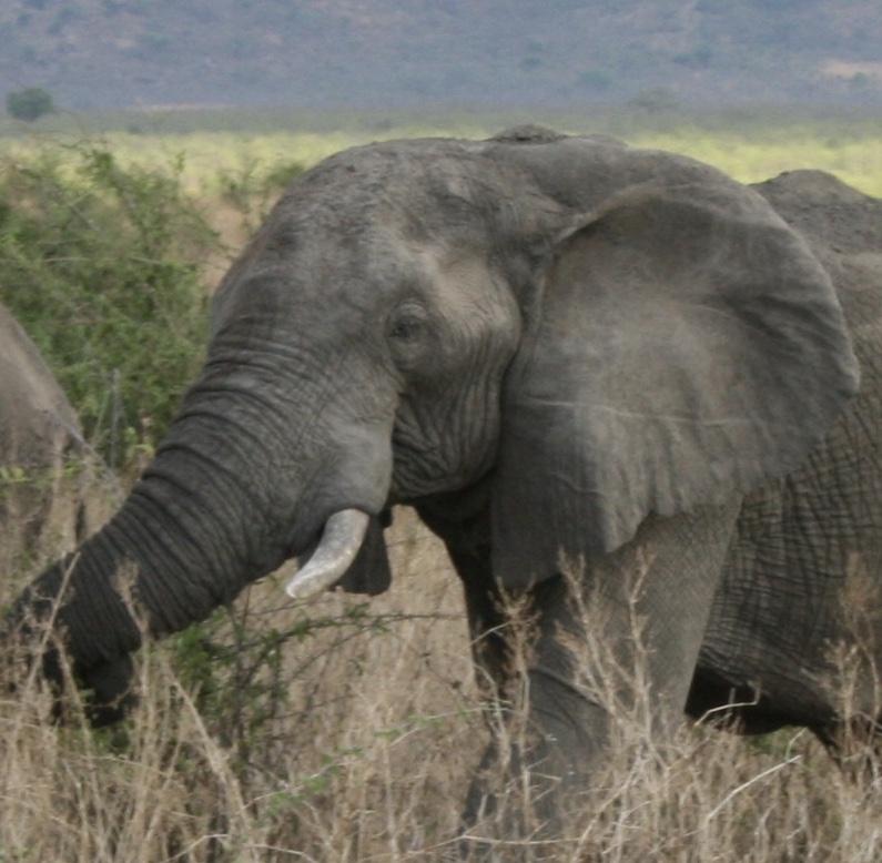
Let’s consider a population of wildebeest with a \(r = 0.016~{\rm month}^{-1}\). This means that - on average - each individual in the population produces 0.016 individuals per month (remember… this accounts for both births and deaths).

Discussion

1. What is \(r\) if the units are \([1/year]\)?
2. Assuming continuous population dynamics, what is the doubling time for this population in terms of months? In terms of years? In terms of centuries?

Remember how to change units! We can use a helpful method that is commonly employed in chemistry. We write out the unit conversions in sequence, ensure that each cancels the other out, resulting in the unit conversion we want. Say we have a rate \(r_y\) that is in \([1/year]\) and we want to convert it to \([1/second]\). We would use the following formula

Discussion

1. If \(r_y = 0.2\), what is the population growth rate in units \([1/second]\)? In units of \([1/day]\)?
2. What are the units of \({\rm d}N/{\rm dt}\)?
3. What are the units of \(N(t + \Delta t) - N(t)\)
4. What are the units of \(K\) in the logistic equation for continuous-time populations?

Carrying Capacity

We have shown how discrete-time population growth relates to continuous-time population growth. We are now going to stick with continuous time population dynamics (we will spend an entire section next week back in discrete time).

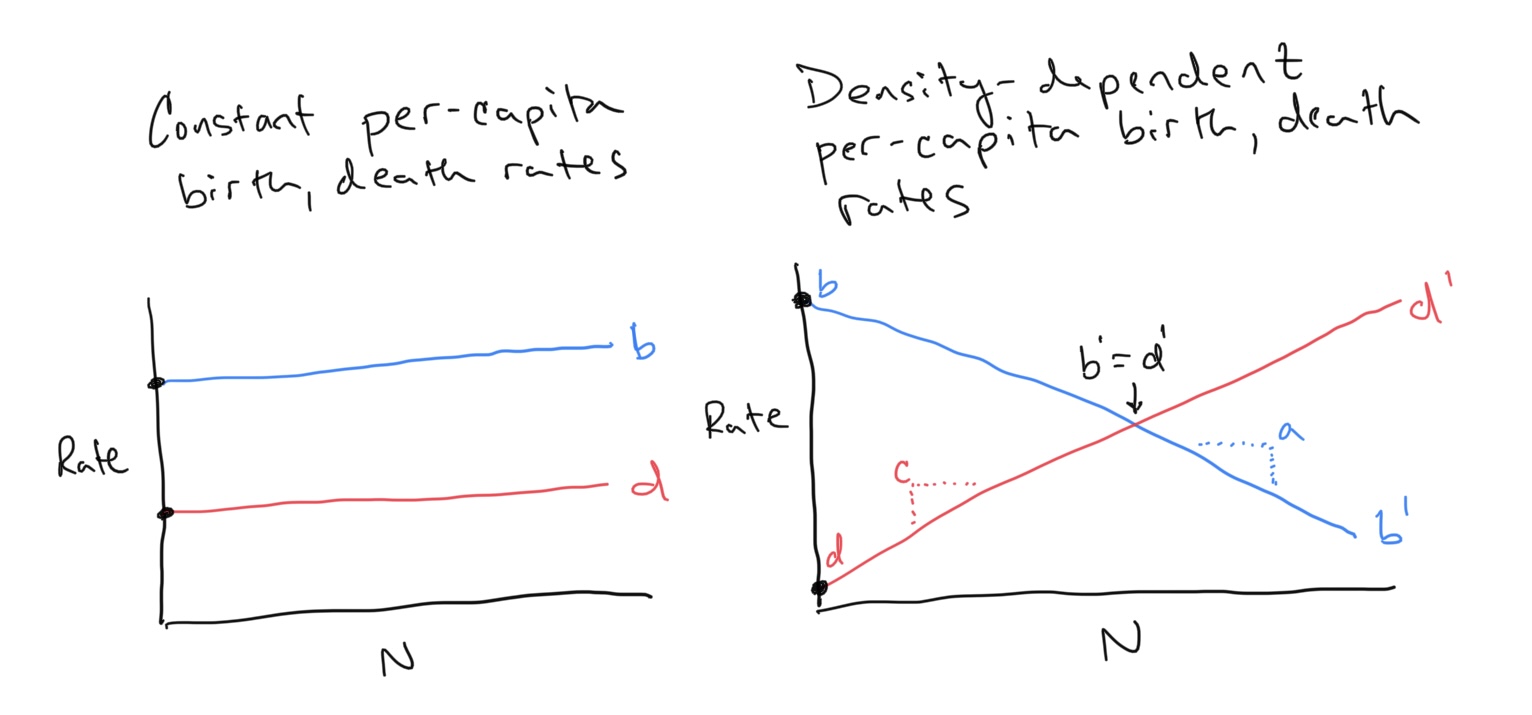
Exponential population growth occurs when the environment and resources are not limiting, and is usually observed at the beginning of a species’ colonization/invasion of a new habitat. However, as the population grows individuals consume resources and space. Eventually this feeds back to influence the rate at which the population is growing. In terms of our equation for population growth, we can say that the per-capita birth and death rates might be expected to change as the environment fills up with individuals. So where before we said total births \(B\) and deaths \(D\) were density-dependent (linear function of \(N\) with slopes given by constant per-capita birth and death rates \(b\) and \(d\)), now we are saying that these per-capita birth and death rates should not be constant, but also change with population size \(N\).

Discussion

1. These population equations generally only track females within sexually-reproducing populations. Why?
2. Why did we choose birth rates to decrease with increasing \(N\) and death rates to increase with increasing \(N\)?
3. For the figures shown on the left and right, we have drawn how per-capita birth and death rates change (or not) as a function of population size. Similar to how we related the fitness of a morph to changes in its proportion within a population, we can reconstruct the flow of the population along the x-axis by observing the relationship between per-capita birth and death rates. When should flow increase and when should flow decrease? Remember that the x-axis is population size \(N\). We are asking when should the population increase and when should it decrease given some combination of per-capita birth and death rates. On the figures above can you use the concept of flow to predict what will happen to the populations?
4. What if we swapped the definitions for birth and death rates? Can you use the concept of flow to anticipate what will happen to the population?

As we will (or have?) explore(d) in class, we can write down equations for density-dependent per-capita birth and death rates as

This explicitly encodes the idea that births decease with increasing \(N\) and deaths increase with increasing \(N\). Note also that the y-intercept for the per-capita birth rate is \(b\) and that the y-intercept for the per-capita death rate is \(d\). In other words, when \(N\) is close to zero (i.e. the population is very very small), the per-capita birth rate \(b^\prime \approx b\) and the per-capita death rate \(d^\prime \approx d\) (where \(\approx\) means is approximately or is close to). As we have defined \(r = b - d\), we can define a density dependent \(r^\prime = b^\prime - d^\prime\).

Let’s substitute this into the continuous-time equation for population growth:

…and to remind us of the meaning of these parameters:

• \(r\) = intrinsic rate of growth (now specifically when the population is small)
• \(b\) = per-capita birth rate when the population is small
• \(d\) = per-capita death rate when the population is small
• \(a\) = the slope at which births decline with increasing population size
• \(c\) = the slope at which deaths incline with increasing population size

Discussion

1. Use algebraic manipulation to derive the 4th equation in the list above from the 3rd equation

We can simplify this a little bit. Let’s define a new parameter

Substituting this term in above gives us

Now let’s investigate how changes in \((r,b,d,a,c)\) impact the dynamics of the system in exactly the same way that we did before with respect to individual fitness. However, instead of visualizing which phenotypic fitness measure was greater or less than the other, we will examine when per capita birth rates are greater than death rates (population growth) and when per capita death rates are greater than birth rates (population decline).

    # Define the Rates function
    pop.flow = function(r,b,d,a,c) {

        # Population size
        N = seq(0,100,5)
        
        # Define per-capita birth and death rates
        pcbr = b - a*N
        pcdr = d + c*N

        # Plot percapita birth and death rates as a function of N
        plot(N,pcbr,type='l',col='blue',lwd=2,ylim=c(min(c(pcbr,pcdr)),max(c(pcbr,pcdr))),xlab='Population Size (N)',ylab='Rate')
        lines(N,pcdr,col='red',lwd=2) 
        legend(0.8,max(c(pcbr,pcdr)),c('p-c birth rate','p-c death rate'),pch=15,col=c('blue','red'))

        # Add flow information
        text(1,(1-0.25)*min(c(pcbr,pcdr)),'Flow',cex=1.5)
        for (i in 1:length(N)) {
            loc = i
            if (pcbr[loc] > pcdr[loc]) {
                text(N[i],min(c(pcbr,pcdr)),'>',cex=1.5)
            } 
            if (pcbr[loc] < pcdr[loc]) {
                text(N[i],min(c(pcbr,pcdr)),'<',cex=1.5)
            }
            if (pcbr[loc] == pcdr[loc]) {
                text(N[i],min(c(pcbr,pcdr)),'--',cex=1.5)
            }
        }
    }
    # Plug in parameter values and run
    pop.flow(r = 0.01,b = 0.8, d = 0.2, a = 0.01,c = 0.01)

Discussion

1. Given r = 0.01,b = 0.8, d = 0.2, a = 0.01,c = 0.01, where does the flow indicate that the population will settle?
2. Plug in the values \((b,d,a,c)\) to solve for \(K\) given the equation for \(K\) above. Comparing this value to what we observe in the graph, what is our interpretation of what \(K\) means?
3. Let’s a) switch b and d and reverse the direction of the slope, so that our parameters are r = 0.01,b = 0.2, d = 0.8, a = -0.01,c = -0.01. How do we interpret what will happen to this population? Is this realistic?
4. Derive the y-intercepts and x-intercepts for \(b^\prime\) and \(d^\prime\) in terms of \((b,d,a,c)\). Can you confirm analytically the x- and y-intercepts that you observe in the above graph?

We are now going to use a differential equation solver to examine how \(N(t)\) changes over time \(t\). This is a numerical method for observing the dynamics of a differential equation system without having to solve for \(N(t)\). In fact, we can solve for \(N(t)\) using integration by parts (shudder), but we won’t go there in this class.

    library(deSolve)
    # Define the logistic growth dynamic model
    pop.logistic = function(r,b,d,a,c,tmax,N0) {
        yini = c(N = N0)
        
        fmap = function (t, y, parms) {
        with(as.list(y), {
            dN <- (b-d)*N*(1 - ((a+c)/(b-d))*N)
            list(dN)
        })
        }
        
        times <- seq(from = 0, to = tmax, by = 0.1) 
        out   <- ode(y = yini, times = times, func = fmap, parms = NULL)
        
        plot(out, lwd = 2,xlab='Time',ylab='Population N(t)')
    }
    # Plug in parameter values and run
    pop.logistic(r = 0.01,b = 0.8, d = 0.2, a = 0.01,c = 0.01,tmax = 1000,N0 = 1)

Discussion

1. Input the initial parameter combinations that we investigated in the flow diagram. How does this plot compliment our expectations of the dynamics from predicting the flow?
2. Unlike the flow diagram, we have to input an initial population size \(N_0\). Try entering a large \(N_0\) as the starting population. What do you observe? Does the long-term dynamics change?
3. What is the role in r? How does changing r change what happens to the population?
4. As before, let’s a) switch b and d and reverse the direction of the slope, so that our parameters are r = 0.01,b = 0.2, d = 0.8, a = -0.01,c = -0.01, tmax = 1000,N0 = 1. Try this for \(N_0 = 1\), \(N_0 = 29\), \(N_0 = 30\), and \(N_0 = 31\). Does what you observe match your expectations for what you predicted the population to do from the flow diagram? Why do you think you got an error message for \(N_0 = 31\)?

Finally, let’s check out a simplified version of what we have above. Instead of changing \((b,d,a,c)\), we will used the compressed notation, where we assess population dynamics in terms of \((r,K)\).

    library(deSolve)
    pop.logistic2 = function(r,K,tmax,N0) {
        yini = c(N = N0)
        
        fmap = function (t, y, parms) {
        with(as.list(y), {
            dN <- r*N*(1 - (N/K))
            list(dN)
        })
        }
        
        times <- seq(from = 0, to = tmax, by = 0.1) 
        out   <- ode(y = yini, times = times, func = fmap, parms = NULL)
        
        plot(out, lwd = 2,xlab='Time',ylab='Population N(t)')
    }
    pop.logistic2(r = 0.01,K = 30,tmax = 1000,N0 = 1)

Discussion

1. Try alternative values for r and K. How do these parameters impact the dynamics of the population when you start at different population sizes N0?

Flow Diagram for the Logistic Equation

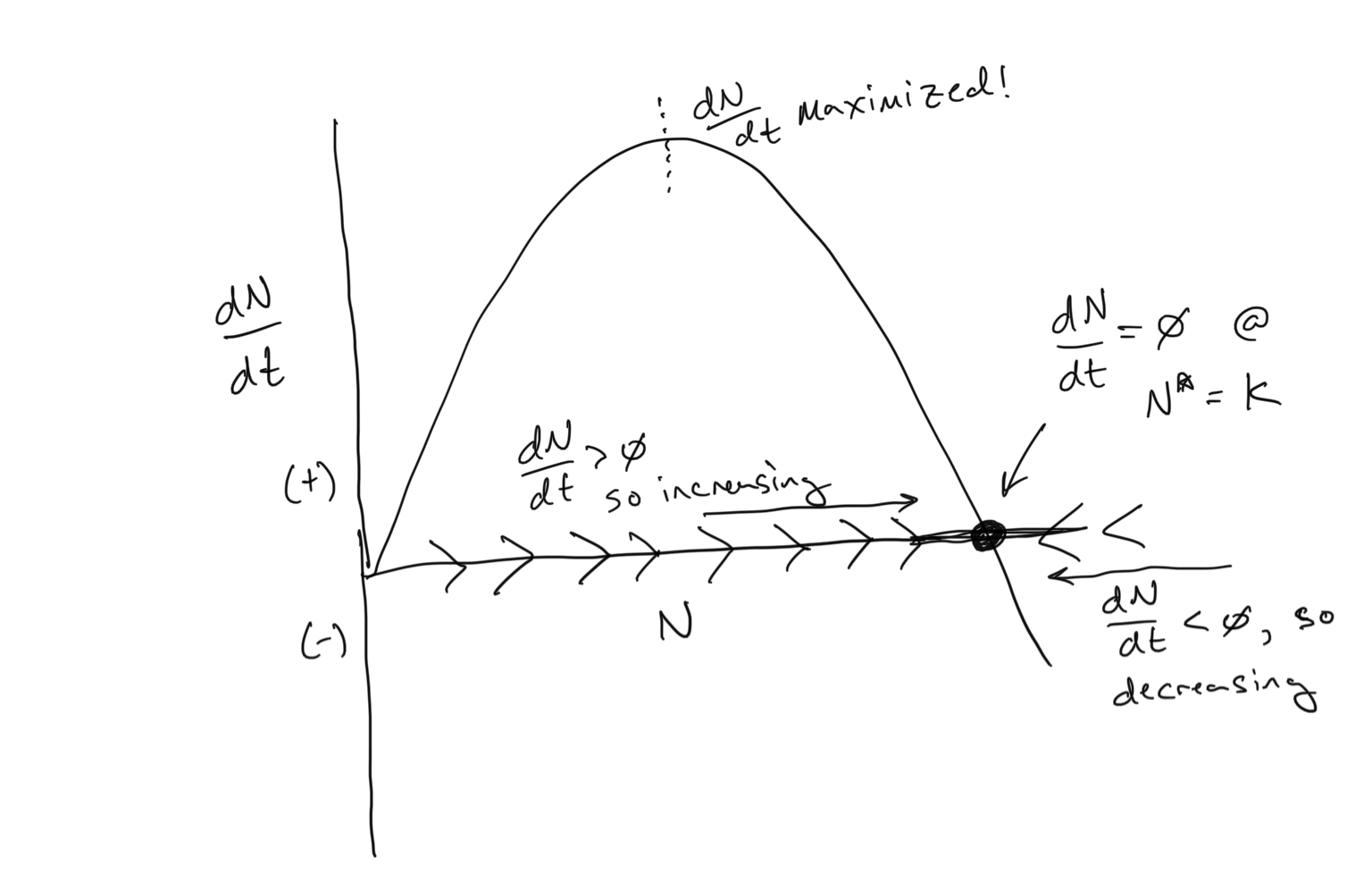
Our population growth equation that incorporates density-dependent per-capita birth and death rates is known as the Logistic Equation. You can see above how it has a sigmoidal shape… population growth begins exponentially but then tapers off as it reaches the carrying capacity \(K\). And we have used the per-capita birth and death rates to anticipate the dynamics using the flow concept. Below we see that we can use the flow concept in a different way… to examine \(dN/dt\) as a function of \(N\).

Discussion

1. Where is the carrying capacity \(K\)?
2. There are two values of \(N\) where \(dN/dt = 0\). What are they?
3. Where is \(dN/dt\) maximized on the plot above? Can you guess the value of \(N\) corresponding to where \(dN/dt\) is maximized? What is special about this point in terms of how the population changes over time?
4. Bonus round: Can you analyitically solve for the point at where \(dN/dt\) is maximized in terms of \(N\)? Hint: to do this you would need to take the derivative of something…

Part II: Discrete Population Growth

Continuous Back to Discrete!

Now let’s decouple the time-step size in the first equation with the goal of turning it into a discrete process. First, we should define \({\rm d}/{\rm dt}\)…

where the \(\lim\) notation means that we are evaluating the function at the limit of \(\Delta t \rightarrow 0\) (this is a foundational concept in Calculus… it means we are assuming the size of the time step is really really really small), and where we specify that the growth rate here is with respect to a (now) discrete-time system via the subscript \({}_d\). Now let’s imagine that \(\Delta t\) is not really really really small such that the \(\lim_{\Delta t \rightarrow 0}\) can be ignored… in fact, let’s assume that \(\Delta t\) is quite large. Because it is large, it’s significance is important, and we will multiply it to both sides of the equation to obtain

To obtain an equation for \(N(t)\) for a discrete time system, we use recursion, which we discussed in class. Following the procedure outlined in lecture we obtain

where \(\lambda = N(t+1)/N(t)\).

Discussion

1. Relate \(\lambda\) to the instantaneous rate of growth \(r\). In other words, solve for \(\lambda\) in terms of \(r\), and solve for \(r\) in terms of \(\lambda\). *Hint: do this by utilizing both continuous- and discrete-time definitions for \(N(t)\).
2. What does \(\lambda\) represent compared to \(r\), and how do different values of each correspond to increasing, decreasing, and steady state population dynamics? Plug in some values for each and experiment.
3. If \(r = 0.02~{\rm year}^{-1}\), what is \(\lambda\) in a corresponding discrete-time system?
4. What are \(r\) and \(\lambda\) at steady state? I.e. at the condition where the change in population size is zero over time?
5. We discussed in class how to calculate the doubling time for a population according to continuous-time dynamics. Using the discrete time solution for \(N(t)\), what is the equation for doubling time for a discrete-time population? How does this compare to the doubling time of a continuous-time population? Hint: Solve \(2N_0 = N_0 \lambda^t\) for \(t\).

Discrete logistic population growth

We have spent a significant amount of time in class deriving the Logistic Population equation for continuous-time dynamics. Now let’s explore a discrete-time version of the logistic equation. For your reference, both the continuous-time (top) and discrete-time (bottom) versions of the logistic equation are presented below.

Think carefully about the differences, and remember that \(N(t+1) - N(t) = \Delta N\), or ‘the change in \(N\). Also note that here \(\Delta t = 1\). Let’s consider whether our expectations for the discrete logistic should be the same or different than the continuous logistic.

Discussion

1. What should \(\Delta N\) approximate if \(N \approx 0\)? Compare this to the same expectation for the continuous-time \({\rm d}N/{\rm dt}\).
2. Do the same for \(N \approx K\).

Okay… so let’s now see if our expectations match reality. Below is a code block where the discrete logistic is simulated over time. As with the continuous-time population equation, we have to supply the initial population size \(N_0\), and the (in this case) discrete growth parameter \(r_d\) and the carrying capacity \(K\). In addition we have to specify the number of time-steps over which we will simulate tmax.

For simplicity, let’s keep K=1 for now. Recall that in class, \(N^* = K\), which means that the steady state for the continuous-time system is at the carrying capacity \(K\). But if \(K=1\), what does this mean? The steady state is at 1 individual??? No - this wouldn’t make sense. Remember that \(N\) could be in units of \([individuals]\) (where only integer values make sense) or could be in units of density \([individuals/area]\). In the case of the latter, fractional values have meaning… for example, let’s consider 0.1 individuals/area. If our area is in units of \([{\rm km}^2]\), 0.1 \(individuals/km^2\) means that there is roughly 1 individual per 10 \({\rm km}^2\). If \(K=1\), then we can assume that we are dealing with densities.

Run the code block below, and see if your expectations for \(N \approx 0\) and for \(N \approx K\) are correct, where in this case \(K=1\).

    logistic.map = function(rd,K,N0,tmax) {
        N = numeric(tmax)
        N[1] = N0
        for (t in 2:tmax) {
            Nt = N[t-1] + rd*N[t-1]*(1 - N[t-1]/K)
            N[t] = Nt 
        }
        plot(N,type='l')
    }

    logistic.map(rd = 1, K = 1,N0=0.01,tmax=30)

Discussion

1. Now set rd = 2. What dynamics do you observe? Describe them. Are they stable?
2. Set rd = 2.5. What dynamics do you observe? Describe them. Are they stable?
3. Set rd = 3.0. What dynamics do you observe? Describe them. Are they stable? Not clear? Change tmax = 100 to give you a longer-time perspective. How would you describe what you see?

Cobweb Diagrams

For the continuous-time logistic equation, we were able to learn a lot about the dynamics of the system by graphically analyzing the ‘flow’ when we plotted \({\rm d}N/{\rm dt}\) (on the y-axis) versus \(N\) (on the x-axis). There is an analogous method for the discrete time logistic equation, however there is a little more to it that requires careful consideration.

For the discrete-time system, we will graphically analyze the plot of \(N(t+1)\) (on the y-axis) as a function of \(N(t)\) (on the x-axis). As with the continuous-time equation, this produces a parabola. The parabola represents the mapping from \(N(t)\) to \(N(t+1)\). In other words, if our population is at value \(N(t)\), to find the next value at time \(t+1\), we identify the value of \(N(t)\) on the x-axis, draw a vertical line up to the parabola, and this gives us the value at \(N(t+1)\). We then reiterate the process. We can make life simpler for ourselves if we also draw the 1:1 line in the same plot (where \(N(t) = N(t+1)\)). Instead of going back to the x-axis for every \(N(t)\) to draw the vertical line up to the parabola (giving us \(N(t+1)\)), we can simply draw a horizontal line to the 1:1 line (resetting \(N(t+1)\) to \(N(t)\)), and than a vertical line up or down to the parabola to get at the next value of \(N(t+1)\). Below we observe the process for tracing the dynamics of a discrete time system in this way:

• First, find \(N(t)\) on the x-axis
• Draw a vertical line up to the parabola. This is \(N(t+1)\)
• Draw a horizontal line over to the 1:1 line. This resets \(N(t)\) along the x-axis
• Draw a vertical line up or down to the parabola. This gives us \(N(t+1)\)
• Draw a horizontal line over to the 1:1 axis
• Repeat, repeat, repeat!

The above algorithm constitutes what we call a cobweb diagram. We implement this algorithm via simulation in the code block below. Run the same parameter sets that you encoded above into the cobweb diagram below. Make sure you understand what the cobweb diagram is showing. Confirm that the time-simulation of the discrete-logistic equation and the cobweb diagram are telling us the same thing.

    logistic.cobweb = function(rd,K,N0,tmax) {
        N = numeric(tmax)
        N[1] = N0
        for (t in 2:tmax) {
            Nt = N[t-1] + rd*N[t-1]*(1 - N[t-1]/K)
            N[t] = Nt 
        }
        Ntx = seq(0,max(N)*(1+0.5),length.out=100)
        Nty = Ntx + rd*Ntx*(1 - Ntx/K)
        xymax = max(N)
        plot(Ntx,Nty,type='l',xlab="Population size N(t)", ylab="Population size N(t+1)",lwd=2,xlim=c(0,xymax),ylim=c(0,xymax))
        lines(seq(-1,2),seq(-1,2),col='gray',lwd=2)
        for (t in 1:(tmax-1)) {
            #draw segments
            segments(x0=N[t],y0=N[t],x1=N[t],y1=N[t+1],col='blue')
            segments(x0=N[t],y0=N[t+1],x1=N[t+1],y1=N[t+1],col='blue')
        }
    }
    logistic.cobweb(rd = 1, K = 1, N0=0.01, tmax=40)

Discussion

1. Across intervals of 0.1, at what value of \(r_d\) do the dynamics become cyclic? Unpredictable?
2. Compare rd=1.8 to rd=2.0. What is the primary difference between these outcomes. Compare both the results of the cobweb diagram and the \(N(t)\) vs. \(t\) plot to establish your interpretation of what is going on.
3. Do we observe cycles or chaotic dynamics in the continuous-time logistic model? (Below is the code block from Section 7 where we assessed continuous-time logistic dynamics, which you can use for reference)
4. Given these differences, what are the long-term implications for discrete-time vs. continuous-time population dynamics?
5. What ecological factors might promote continuous- vs. discrete-time population dynamics?

Compare the Continuous- and Discrete-time systems directly

This code block allows us to directly compare the temporal dynamics of continuous-time and discrete-time logistic populations directly. Use this to inform your answers to the above questions.

    library(deSolve)
    pop.combined = function(r,K,N0,tmax) {
        #Continuous model
        yini = c(N = N0)
        fmap = function (t, y, parms) {
        with(as.list(y), {
            dN <- r*N*(1 - (N/K))
            list(dN)
        })
        }
        
        times <- seq(from = 1, to = tmax, by = 0.1) 
        out   <- ode(y = yini, times = times, func = fmap, parms = NULL)
        
        # Discrete model
        Nd = numeric(tmax)
        Nd[1] = N0
        for (t in 2:tmax) {
            Ndt = Nd[t-1] + r*Nd[t-1]*(1 - Nd[t-1]/K)
            Nd[t] = Ndt 
        }
        maxN = max(c(Nd,out[,2]))
        plot(out, lwd = 2,xlab='Time',ylab='Population N(t)',col='blue',ylim=c(0,maxN))
        lines(Nd,col='red',lwd=2)
    }
    pop.combined(r = 1,K = 1,N0 = 0.01,tmax = 40)