Section 2: Temperature as an ecological constraint
Environmental constraints on organismal function and behavior
As we are learning in Chapters 4 & 5 of the textbook, where species live and how they function is strongly constrained by the environmental conditions - in particular water and temperature. In this Discussion Section, we will explore how temperature constrains the behaviors of lizards. Lizards are ectotherms (i.e. “cold-blooded”), which means that they do not regulate their own body temperatures, relying instead on the environment to regulate their temperature for them. The performance of key physiological processes depend on temperature… if the temperature is too low or too high, these processes perform suboptimally. This means there is a sweet-spot temperature where performance is optimized, and this sweet-spot differs from species to species. In contrast to ectotherms, endotherms spend extra energy to maintain their internal body temperature. This is why, when you take your temperature, you generally register around 98.5° Fahrenheit.
Discussion
- What are some physiological processes that are temperature-dependent?
- Physiology is an enormously complex dance of chemical reactions which are all dependent on temperature. What are some organismal activities that might be impacted by changes in temperature?
- What are the benefits/drawbacks of ectothermy/endothermy?
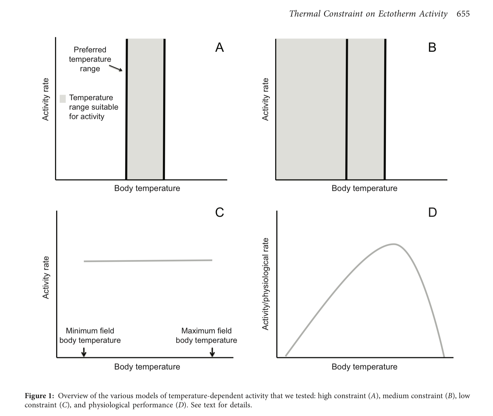
A model is a simplified expression of a natural phenomenon(a), designed to capture the most important elements of a complex problem, thereby promoting understanding. A simple model of organismal activity budgets can be a powerful tool to understand how changes in the environment may impact species, and can enable ecologists to build predictions for how species might react to environmental changes anticipated to occur with climate change. In the figure below we can see 3 models A (high-constraint model), B (medium-constraint model), C (low-constraint model). Panel D illustrates the idea that - in reality - physiological processes (and resultant activbity patterns) are expected to change continuously with temperature, but capturing this with a model that is extendable to many species is very difficult.
Discussion
- Compare and contrast each model with each other
- What simplifications and assumptions do each of the models make? Which of the models are simpler and which are more complicated?
- Why would it be very difficult to establish a general model that captures the idea illustrated in Panel D that is applicable to many species?
Patterns of Thermal Constraint on Ectotherm Activity
In 2015, Alex Gunderson and Manuel Leal (Duke University) published a paper where they examined which of these four proposed models best captured reality for Anolis lizards in Puerto Rico. Anolis cristatellus is an arboreal lizard that is endemic to the islands of the Greater Puerto Rican Bank. By conducting field observations of these lizards, the scientists wanted to capture how lizard activity patterns varied with local temperatures. For that, they had to a) make careful observations of activity patterns and b) assess local temperatures (which might be very different than regional temperatures, as they must account for microclimates). Activity rate was defined by the proportion of observational time a lizard was engaging in agonistic encounters, feeding events, mating, and signaling displays.
“Focal lizards were located by walking slowly through the forest along transect lines that followed randomly generated compass directions and starting in a different hap-hazard location every day. This method made it extremely unlikely that a given individual was observed more than once, and it allowed us to sample large areas of each forest.”
After they collected data on how activity patterns varied with temperature, they could compare their observed results with simulations conducted according to the constraints imposed by each of the proposed models. The simulation results that most closely match the scientists’ observations should point to the model that best captures reality. We will not be discussing the simulation models, but we will examine how these simulation results matched or did not match what the scientists observed in nature
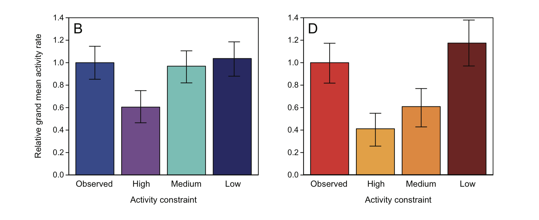
The panel on the left shows have each of the model results compare to those observed in mesic (wet) habitats; the panel on the right shows how each of the model results compare to those observed in xeric (dry) habitats.
Discussion
- Is there a stand-out model that captures reality better than the others?
- Which models do better/worse?
Analyzing the observational data
Now we will use R to examine the data that the authors gathered directly. We will use the web-tool a bit differently this time, because there is a lot of data that we might want to look at in different ways, and we don’t want to cut/paste the data in the web-tool every time. Below you will see a code block with the raw data, and the web-tool below. Cut and paste the data entry code into the web tool.
Below the comment # Evaluation, we will paste code to plot the data in various ways. Below the web-tool there is an # Evaluation tools code block. For each step of the Evaluation code block, replace the evaluation commands in the web-tool and press RUN. Follow the directions written in the comments of the Evaluate tools code block.
    activity = c(0.069, 0.01, 0.014, 0.11, 0.158, 0.169, 0.122, 0.122, 0.052, 0.008, 0.024, 0.146, 0.025, 0.044, 0.242, 0.143, 0.253, 0.203, 0.563, 0.006, 0.092, 0.151, 0.525, 0.324, 0.411, 0.306, 0.745, 0.492, 0.205, 0.192, 0.016, 0.301, 0.247, 0.002, 0.012, 0.405, 0.125, 0.064, 0.248, 0.124, 0.468, 0.205, 0.168, 0.595, 0, 0.143, 0.019, 0.046, 0.079, 0.174, 0.163, 0.133, 0.006, 0.234, 0.094, 0.439, 0.018, 0, 0.045, 0.127, 0.173, 0.21, 0, 0.009, 0.108, 0.14, 0.275, 0.037, 0.212, 0.196, 0.147, 0.097, 0.152, 0, 0.061, 0.251, 0.31, 0.181, 0.368, 0.307, 0.407, 0.094, 0.312, 0.017, 0.082, 0.036, 0.47, 0.198, 0.099, 0.064, 0.232, 0.112, 0.188, 0.311, 0.289, 0.201, 0.081, 0.055, 0.004, 0.048, 0.167, 0.003, 0.116, 0, 0.007, 0.002, 0.069, 0.026, -0.009, 0, 0.004, 0.05, 0.29, 0.062, 0.307, 0.006, 0.059, 0.025, 0.148, 0.118, 0.052, 0.005, 0.112, 0.081, 0.2, 0.155, 0.251, 0.188, 0.129, 0.092, 0.055, 0.208, 0.169, 0, 0.02, 0.065, 0.143, 0.087, 0.007, 0.014, 0.479, 0, 0.2, 0.042, 0.034, 0.152, 0.077, 0.325, 0.052, 0.045, 0.253, 0.244, 0.055, 0.139, 0.01, 0.06, 0.094, 0.018, 0.108, 0.02, 0.02, 0.038, 0.209, 0.134, 0.194, 0.286, 0.061, 0.062, 0.223, 0.057, 0.116, 0.102, 0.432, 0.206, 0.079, 0.576, 0.074, 0.026, 0.133, 0.183, 0.197, 0.138, 0.4, 0.339, 0.332, 0.003, 0.052, 0.047, 0.101, 0.063, 0.079, 0.059, 0.032, 0.202, 0.427, 0, 0.076, 0.003, 0.102, 0.086, 0.354, 0.099, 0.224, 0.111, 0.04, 0.048, 0.176, 0.006, 0.063, 0.524, 0.255, 0.153, 0.173, 0, 0.141, 0.017, 0.085, 0.33, 0.385, 0.21, 0.259, 0.211, 0.105, 0.399, 0.014, 0.302, 0.311, 0.155, 0.831, 0.482, 0.245, 0.009, 0.043, 0.591, 0.1, 0.006, 0.095, 0.323, 0.257, 0, 0.151, 0.014, 0.037, 0.119, 0.343, 0.1, 0.067, 0.091, 0.02, 0.154, 0.067, 0.211, 0.087, 0.263, 0.019, 0.226, 0.53, 0.16, 0.359, 0.145, 0.058, 0.351, 0.018, 0.219, 0.05, 0.105, 0, 0.235, 0.089, 0.2, 0.163, 0.216, 0.268, 0.206, 0.148, 0.055, 0.353, 0.012, 0.106, 0.188, 0.04, 0.34, 0.036, 0.028, 0.137, 0.147, 0.044, 0.351, 0.269, 0.372, 0.117, 0.11, 0.258, 0.053, 0.428, 0.098, 0.018, 0.354, 0.044)

    temp = c(29.9, 30.8, 30.9, 30.4, 30.4, 30.5, 32.4, 32.4, 32.8, 31.5, 29.9, 30.9, 28.9, 31, 30.3, 32.3, 32.7, 34.8, 35.9, 32.2, 31.3, 31.5, 32.3, 31.6, 30.2, 30.7, 28.3, 30.5, 32.4, 29.9, 31.9, 31.7, 33.1, 32.7, 32.4, 33.3, 34.5, 33, 33.2, 31.8, 30.9, 31.3, 30.3, 30.7, 26.7, 27, 28, 27.9, 27.7, 27.1, 27.5, 28.3, 28.3, 28.9, 27.8, 28.9, 28, 27.3, 27.9, 28.9, 30.8, 30.6, 32, 32.7, 33.6, 28.9, 29.3, 29.7, 30.2, 30.7, 30.3, 31.7, 33.3, 32.4, 32.2, 31.2, 30.4, 30.4, 30.4, 31.9, 31.6, 30.7, 30.7, 30.3, 27.6, 29.5, 29.7, 30, 30, 29.9, 27.8, 27.7, 27.7, 28.4, 28.1, 28.2, 27.6, 28.6, 25.8, 27.4, 27.1, 30.1, 28.7, 28, 30.1, 29.4, 33.5, 29.6, 29.4, 31.2, 26.6, 26.7, 28.6, 26, 26.2, 27.1, 27.2, 28.3, 31, 31.1, 28.8, 30.1, 27.1, 27.7, 28, 30.6, 29.6, 29.4, 30.9, 31.2, 31.6, 32.6, 33.3, 33.1, 33.2, 32.2, 32.2, 32.4, 32.2, 32.3, 31, 27.7, 27.8, 27.6, 28, 28.3, 29.2, 29.2, 29.2, 29.3, 29.6, 29.3, 29.3, 29.3, 29.1, 29.2, 28.7, 28.2, 28.6, 28.1, 27.2, 28.2, 27.8, 27.7, 28, 29.4, 29.1, 29.8, 29.9, 29.8, 29.6, 27.6, 26.9, 26.8, 27.1, 27.1, 27.7, 27.4, 27.3, 28.3, 29.1, 29.4, 29.6, 29.5, 29.6, 30.5, 30.4, 30.8, 31.3, 30.7, 29.6, 30.2, 29.4, 29.2, 28.5, 26.1, 26.7, 27.1, 27, 27.4, 27.6, 28.2, 29.4, 28.8, 29.1, 30.1, 29.6, 30, 29.3, 28.7, 28.2, 28, 27.7, 28.1, 27.1, 27.8, 28.3, 28, 27.7, 29.3, 29.7, 29.6, 30, 30.3, 30.3, 30.3, 30.2, 29.9, 28.7, 28.5, 28.3, 27.8, 28.3, 28.6, 25.7, 26.6, 27.2, 27.6, 28.8, 29.5, 29.8, 30.1, 30.8, 31.1, 31.9, 31.6, 30.4, 31.4, 30.2, 30.4, 29.9, 29.8, 29.6, 28.6, 27.1, 27.4, 28.1, 28.2, 28.4, 28.3, 27.8, 28.6, 29.2, 29.4, 29, 27.7, 27.7, 27.9, 28.9, 28.8, 28.9, 29.8, 30.4, 30.1, 29.8, 29.7, 29.6, 28.9, 29.4, 29.2, 27.7, 28, 28.5, 27.7, 28.9, 29.1, 29.1, 29.6, 29.9, 28.7, 28.9, 29.5, 29.2, 28.7, 29, 29.1, 29.4, 28.4, 28.4)

    # 1 = female; 2 = male
    sex = c(2, 1, 1, 2, 2, 2, 2, 2, 1, 1, 2, 2, 1, 1, 2, 2, 1, 1, 2, 1, 2, 2, 1, 2, 1, 1, 2, 2, 1, 1, 1, 1, 2, 2, 1, 1, 2, 2, 1, 2, 2, 1, 1, 2, 1, 2, 2, 1, 2, 1, 1, 2, 1, 2, 1, 1, 1, 2, 1, 2, 1, 1, 2, 2, 1, 1, 1, 2, 2, 1, 2, 1, 2, 1, 1, 2, 1, 1, 2, 1, 2, 1, 2, 1, 1, 1, 2, 1, 2, 1, 2, 1, 1, 2, 2, 1, 2, 2, 1, 2, 1, 1, 2, 2, 2, 1, 2, 1, 1, 2, 2, 2, 2, 2, 2, 2, 1, 1, 1, 2, 1, 2, 1, 1, 2, 2, 2, 1, 2, 1, 1, 2, 2, 1, 1, 2, 2, 2, 1, 1, 2, 1, 2, 1, 2, 1, 2, 1, 2, 1, 2, 2, 1, 2, 1, 1, 2, 2, 1, 1, 1, 2, 1, 2, 1, 2, 1, 2, 1, 2, 1, 1, 2, 2, 2, 2, 1, 2, 2, 2, 1, 2, 2, 1, 2, 2, 1, 1, 2, 2, 1, 2, 2, 1, 1, 1, 2, 1, 2, 1, 2, 1, 2, 1, 2, 2, 1, 2, 1, 2, 2, 2, 1, 2, 2, 2, 1, 2, 1, 2, 2, 1, 2, 1, 2, 1, 1, 2, 1, 2, 2, 1, 1, 2, 2, 1, 1, 2, 2, 1, 2, 1, 1, 2, 1, 2, 1, 2, 1, 2, 1, 2, 2, 1, 1, 2, 1, 2, 2, 1, 2, 1, 2, 1, 2, 1, 2, 1, 1, 1, 2, 1, 2, 2, 1, 1, 1, 1, 1, 1, 2, 2, 1, 1, 2, 1, 2, 1, 2, 2, 1, 2, 1, 2, 1, 2, 1, 2, 1)

    # 1 = guan (warmer, more variable); 2 = camb (cooler, less variable)
    locality = c(1, 1, 1, 1, 1, 1, 1, 1, 1, 1, 1, 1, 1, 1, 1, 1, 1, 1, 1, 1, 1, 1, 1, 1, 1, 1, 1, 1, 1, 1, 1, 1, 1, 1, 1, 1, 1, 1, 1, 1, 1, 1, 1, 1, 1, 1, 1, 1, 1, 1, 1, 1, 1, 1, 1, 1, 1, 1, 1, 1, 1, 1, 1, 1, 1, 1, 1, 1, 1, 1, 1, 1, 1, 1, 1, 1, 1, 1, 1, 1, 1, 1, 1, 1, 1, 1, 1, 1, 1, 1, 1, 1, 1, 1, 1, 1, 1, 1, 1, 1, 1, 1, 1, 1, 1, 1, 1, 1, 1, 1, 1, 1, 1, 1, 1, 1, 1, 1, 1, 1, 1, 1, 1, 1, 1, 1, 1, 1, 1, 1, 1, 1, 1, 1, 1, 1, 1, 1, 1, 1, 1, 2, 2, 2, 2, 2, 2, 2, 2, 2, 2, 2, 2, 2, 2, 2, 2, 2, 2, 2, 2, 2, 2, 2, 2, 2, 2, 2, 2, 2, 2, 2, 2, 2, 2, 2, 2, 2, 2, 2, 2, 2, 2, 2, 2, 2, 2, 2, 2, 2, 2, 2, 2, 2, 2, 2, 2, 2, 2, 2, 2, 2, 2, 2, 2, 2, 2, 2, 2, 2, 2, 2, 2, 2, 2, 2, 2, 2, 2, 2, 2, 2, 2, 2, 2, 2, 2, 2, 2, 2, 2, 2, 2, 2, 2, 2, 2, 2, 2, 2, 2, 2, 2, 2, 2, 2, 2, 2, 2, 2, 2, 2, 2, 2, 2, 2, 2, 2, 2, 2, 2, 2, 2, 2, 2, 2, 2, 2, 2, 2, 2, 2, 2, 2, 2, 2, 2, 2, 2, 2, 2, 2, 2, 2, 2, 2, 2, 2, 2, 2, 2, 2, 2, 2, 2, 2, 2, 2, 2)

    # Evaluation! (paste code below here to plot/evaluate)
    # Evaluation code

    ##############
    # Analysis 1
    ##############

    # First, let's examine how activity rates varies with temperature
    plot(temp,activity,xlab="Temperature", ylab="Activity rate")

    # This looks like a mess, doesn't it? Is there any pattern that suggests itself?
    # This is also a good lesson to learn early: Ecological data are MESSY.

    ##############
    # Analysis 2
    ##############

    # Let's look for any patterns in the noise. Aside from temperature and activity,
    # we also have the sex and locality information for each lizard evaluated
    # Now let us see if there are differences in the bulk activity measures across sex and location

    # First let's look at LOCATION
    # We will use a boxplot to compare location-dependent differences
    # What are the important elements of a box plot and what do they represent?
    boxplot(list(activity[which(locality==1)],activity[which(locality==2)]),col='gray',boxwex=0.5,names=c("Xeric (dry)","Mesic (wet)"),ylab="Activity rate")

    # Do you observe any differences?

    # Now, let's examine whether there are differences in activity patterns among males/females
    boxplot(list(activity[which(sex==1)],activity[which(sex==2)]),col='gray',boxwex=0.5,names=c("Female","Male"),ylab="Activity rate")

    # Do you observe any differences?

    # Now... it can be quite tricky to say whether two sets of results are
    # *different enough* to be considered different. In Gunderson & Leal's paper
    # they use a statistical test (ANOVA = ANalysis Of VAriance) to determine this.
    # They find that lizards between habitats do NOT show differences in activity patterns,
    # but that male vs. female lizards DO show significantly different activity patterns.
    # Examine these differences again. For the males vs. females, which groups have
    # lower vs. higher activity patterns?

    ##############
    # Analysis 3
    ##############

    # Now we are going to re-examine lizard activity rates as a function of temperature.
    # We are going to fit a curved line through the data points... even though
    # there is a lot of variation in the data, fitting a curved line through the
    # points may reveal a trend in activity rates. This curved line is called a
    # cubic spline. The details of this don't matter for now, except that we are
    # using the data to reveal a central trend in activity rates vs. temperature
    # We are also selecting only activity rates corresponding to temperatures below 34

    # Plot the activity rate vs. temperature as before...
    plot(temp,activity,xlab="Temperature", ylab="Activity rate")
    # This is the code to generate the fitted line through the data
    fit = smooth.spline(temp[which(temp<34)],activity[which(temp<34)],spar=0.9)
    # Now we will draw this line into the plot
    lines(fit,lwd=3)
Discussion
- Why might activity patterns vary by sex but not with respect to locality?
- For the activity rates vs. temperature, what does the fitted curve suggest? Why did we choose to ignore activity rates for temperatures > 34°?
Data suggests a different model to capture activity windows
None of the 3 proposed models (High-, medium-, and low-constraint) does a great job at predicting observed activity rates in both mesic and xeric sites. Of all the models, the low-constraint model does the best. According to Gunderson & Leal, the low-constraint model does quite good for the mesic environment, and overestimates the mean activity rate by 17% in the xeric habitat. This suggest that a model that is intermediate to the High-, medium-, and low- constraint model may be worthwhile to explore.
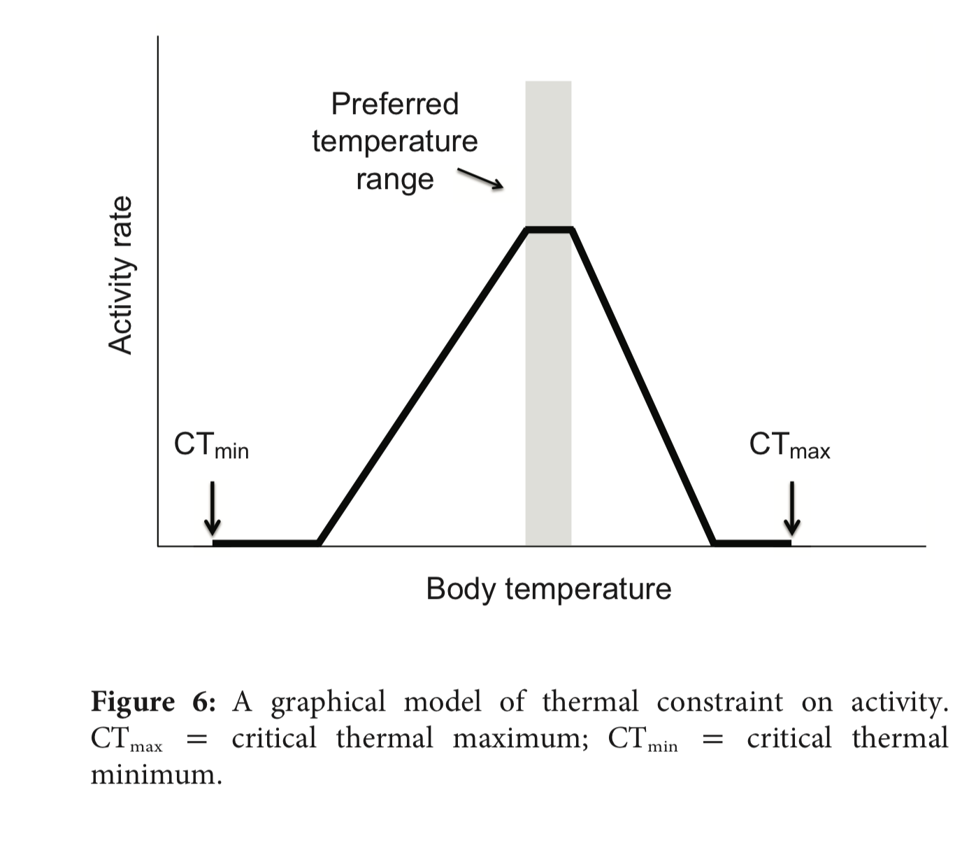
Using the results from Activity 3 in the above analysis, Gunderson & Leal propose the following model to predict activity rates as a function of temperature:
Discussion
- Discuss how this proposed-model of temperature-dependent activity rates is inspired by the observational data that Gunderson & Leal collected.
- How is this model intermediate to the medium- and low-constraint model? What aspects of each does it contain?
Hopefully you can see how ecologists use simple models to build predictions of the natural world, and perhaps more importantly, use observations of natural systems to refine and update those models. This is how science works. We capture our understanding of the natural world with simple relationships, and we call this a model. A model can be verbal, mathematical, graphical, a simulation, etc. We make predictions with the model, and then compare those predictions with observations of the natural world. If we are careful, the natural world will tell us if our model does a good or bad job… either one might be interesting! We then revise our models with our new understanding. Rinse and repeat.