Demo 5 :: Island Biogeography

< Back to Course Page

The Equilibrium Model of Island Biogeography

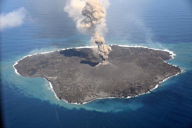
Let’s consider a collection of species living on a mainland. Across a narrow channel sits an island, recently decimated by a volcanic explosion. The lifeforms on the island have been incinerated, and its barren landscape is devoid of anything larger than a few hardy microbes. Now we can begin to imagine different modes of transport available to species on the mainland, and how they might facilitate immigration to the island. Perhaps wind-blown or bird-carried seeds arrive first. Some fast-growing (R-reproductive strategy) weeds might take hold before anything else. Because birds and flying insects come and go as they please, these highly mobile species might begin to roost on the rocks and feast on the newly-grown leaves and seeds produced by the weedy plants. Every once in a while, small mammals, reptiles, and/or land-bound insects accidentally float across the channel when a log they’ve made into their home is pulled out by the tide and happens upon the deserted shores. Very rarely, we might follow an enterprising coyote who swims across the channel, looking for food to eat. The coyote will be disappointed unless there is first established populations of mice, ground squirrels, or the like, to sustain it. Only when these potential prey have established does a coyote successfully make a home. She is female and pregnant, changing the nature of our island community for years to come.

This story has repeated itself in different ways, with different species, in different parts of the world, many many times throughout the history of life on earth. The dynamics of these ecological relationships are captured in a body of theory known as the Theory of Island Biogeography, first detailed by the founder of ecological theory, Robert MacArthur, and his collaborator E.O. Wilson, who just recently passed away. While every island is unique, and every collection of species presents its own distinct character, a body of theory aims to find the underlying similarities that link the dynamics common to all such situations in an effort to generalize and ultimately understand why one island looks one way and another island looks so very different.

The central processes unifying the Theory of Island Biogeography include colonization and extinction dynamics. Colonization details the rate at which species immigrate to an island, and extinction details the rate at which species go extinct. Keep in mind that for this exercise we are not specifying one species from another… so our collection of species, while they involve weedy perennials, shrubs, insects, birds, reptiles and perhaps a few mammals thrown in for good measure, will remain to us just a collection of species with no discernable identifications. However, keep in the back of your mind the story that initiated this activity… the order in which species arrive should matter, even though we will not be considering these important details here.

On the mainland we have a community of \(P\) species (for the species ‘Pool’). We want to build an expectation for how the number of species on the nearby island \(S\) will assemble from this mainland species pool. We can establish a few rules straight away.

• 1) Immigration of species from the pool \(P\) to the island will increase island species richness \(S\).
• 2) Extinction of species on the island will decrease island species richness \(S\)

With this as a starting point, we can build an equation for \({\rm d}S/{\rm d}t\):

Let’s now specify a few parameters. Let’s let \(\lambda_S\) be the number of species immigrating per unit time, and \(\mu_S\) be the number of species going extinct per unit time, so we will rewrite the above equation as

Now let’s think about what these immigration and extinction rates should look like as a function of the number of species on the island. In other words, we want to examine these rates as functions of \(S\), or \(\lambda_S(S)\) and \(\mu_S(S)\). Immigration first. We can write two simple rules and one extrapolation:

• 1) The immigration rate should be zero when the number of species on the island is equal to the number of species in the pool… i.e. \(S=P\).
• 2) When the island is empty, the immigration rate should be maximized (lots of open niches), and as it fills the immigration rate should decline (niches fill up). Let’s call the maximum immigration rate \(I\).
• 3) An extrapolation: to make this model as simple as possible, let’s imagine that the immigration rate linearly decreases from some maximum rate \(\lambda_S=I\) when \(S=0\) to \(\lambda_S = 0\) when \(S=P\).

These relationships give us a linear equation for \(\lambda_S(S)\) over \(S\), in other words

Now that we have established a simple relationship for the immigration rate, we should also think carefully about the extinction rate. Here we can also outline two simple rules and an extrapolation:

• 1) The extinction rate will be zero when there are no species to go extinct! i.e. when \(S=0\).
• 2) The extinction rate will be highest when the island is full. At that point all of the niches are filled and competition can be assumed to be maximized. Let’s call the maximum extinction rate \(E\).
• 3) An extrapolation. Between the lowest number of species \(S=0\) and the greatest number of species \(S=P\), let’s imagine that the extinction rate linearly increases from \(\mu_S = 0\) to \(\mu_S = E\).

These relationships give us a linear equation for \(\mu_S(S)\) over \(S\), and putting everything together yields

Discussion

1. Experiment with the new equation for the immigration rate. Does it give the correct immigration rate across potential values of \(S\)?
2. Experiment with the new equation for the extinction rate. Does it give the correct immigration rate across potential values of \(S\)?
3. We have assumed that \(\lambda_S\) is maximized when \(S=0\). Consider how priority effects might change this assumption. Priority effects describe the idea that the order of species arrival on the island matters.
4. Now you should have a good sense about where we are going for this… Using this equation, what is the equilibrial species richness \(S^*\) for the island community?
5. Using the codeblock below where we simulate \({\rm d}S/{\rm dt}\) and your solution for the equilibrial species richness \(S^*\), see if your expectation matches the simulation of the community over time given specific values for \(P\), \(I\), and \(E\).
6. How does increasing/decreasing \(E\) and \(I\) change your expectations? How does changing \(P\) alter your expectations?
7. Consider how these ideas are similar or dissimilar from predicting population dynamics by way of understanding birth and death rates as a function of population size.

Island Biogeography in the real world

Watching islands fill up I: In 1969, Daniel Simberloff and E.O. Wilson decided to test a theory that Robert MacArthur and Wilson had formulated a few years before: The Theory of Island Biogeography. We will learn more about these ideas during the second half of the class, but here is the gist:

1. Islands represent unique opportunities to test ecological theories… they are as close to a controlled natural experiment as we will ever get.
2. Islands are limited in area and resources, so the number of species that live on islands should also be limited.
3. Such limitations on species richness should be set by a) the size of the island and b) the distance of the island to the mainland (where species will be migrating from)
4. As explored above, the rate at which species arrive on the island (the immigration rate), and the rate at which species go extinct (the extinction rate) are the processes that drive species richness, and these processes should vary as a function of attributes such as island size and distance to the mainland.

Discussion

1. How should the immigration rate change with island size or distance?
2. How should the extinction rate change with island size or distance?

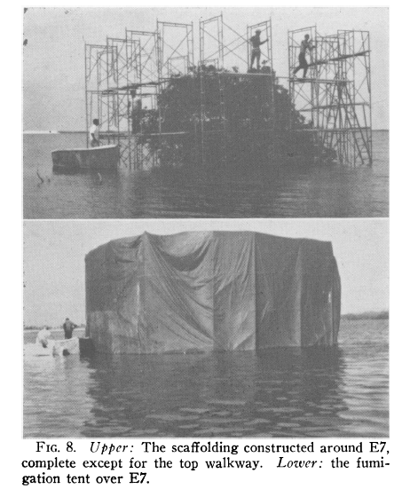
The experiment Simberloff devised is both simple and a bit nutty. He selected a number of mangrove islands off the coast of Florida of varying sizes and distances from the mainland, which hosted diverse arthopod communities. He surrounded each mangrove island with a metal frame, covered it with fumigation tarps, and gassed the arthropods into oblivion. Following these localized ‘mass extinction’ events, Simberloff and colleagues observed the recolonization of the mangrove islands, documenting which species arrived and when. We will now examine these data below.

    # Load in the dataset collected by Simberloff (nicely compiled as a readily availabel package!)
    library(island)
    library(RColorBrewer)
    data = simberloff
    # This is a color palette that shows up well on light backgrounds
    pal = brewer.pal(6,'Dark2')
    
    
    # There are presence/absence datasets for each of 6 islands.
    # Each island is represented by a matrix, where columns are days and
    # rows are species
    # We will add up the number of species present at each time point (island1-6)
    # We will also extract the day the measurements were taken (time1-6)
    # For a given island, we now have a record of how diversity changes over time
    # The first measurement is diversity prior to removal
    # The latter measurements document how the community recovers
    island1 = apply(data[[1]][,2:16],2,sum)
    time1 = as.numeric(names(data[[1]][,2:16])); time1[1] = 0
    island2 = apply(data[[2]][,2:18],2,sum)
    time2 = as.numeric(names(data[[2]][,2:18])); time2[1] = 0
    island3 = apply(data[[3]][,2:17],2,sum)
    time3 = as.numeric(names(data[[3]][,2:17])); time3[1] = 0
    island4 = apply(data[[4]][,2:19],2,sum)
    time4 = as.numeric(names(data[[4]][,2:19])); time4[1] = 0
    island5 = apply(data[[5]][,2:17],2,sum)
    time5 = as.numeric(names(data[[5]][,2:17])); time5[1] = 0
    island6 = apply(data[[6]][,2:16],2,sum)
    time6 = as.numeric(names(data[[6]][,2:16])); time6[1] = 0

    

    # Let's plot these diversity curves for islands 1-6
    # We will use a different color for each island to easier see within-island
    # diversity patterns over time
    plot(time1,island1,type='l',col=pal[1],lwd=2,xlim=c(0,550),ylim=c(0,50),xlab='Time', ylab='Island species richness')
    lines(time2,island2,col=pal[2],lwd=2)
    lines(time3,island3,col=pal[3],lwd=2)
    lines(time4,island4,col=pal[4],lwd=2)
    lines(time5,island5,col=pal[5],lwd=2)
    lines(time6,island6,col=pal[6],lwd=2)
    legend(400,20,legend=c(1,2,3,4,5,6),col=pal,pch=16)

    # We can assess recovery by comparing the species diversity at the first 
    # point in time (pre-extermination) to the species diversity at the last
    # point in time (post-recovery). If we divide the last value by the first
    # value, we get a ratio. A value greater than 1 means that the recovery has
    # resulted in a community MORE diverse than when it started. A value
    # less than 1 means that the recovery has resulted in a community
    # LESS than when it started

    # Let's do this with the first island. We will use the R functions 
    # head() and tail() to get the first and last values
    
    pre_extinction = head(island1,1)
    post_recovery = tail(island1,1)
    ratio = post_recovery/pre_extinction
    print(paste('ratio=',ratio))
    

Discussion

1. What happens to the island communities following Simberloff’s fumigation treatment (the datapoint at time t=0 is species richness before fumigation)
2. What type of variation is observed between and among island communities?
3. What do you think about the ethics of fumigating mangrove islands full of arthropods to examine foundational concepts in ecology? Is there a less impactful way to go about investigating these questions?

Watching islands fill up II: The patterns of community re-assembly following Simberloff’s fumigation are varied, but follow similar trends. One of the principle ideas behind The Theory of Island Biogeography is that:

1. Larger islands should support more species
2. Islands closer to the mainland should support more species

Do we see these relationships with Simberloff’s data? Let’s explore below.

    # Now we will ask the questions: 
    # Do larger islands host richer communities?
    # Do closer islands host richer communities?
    # We will evaluate this with respect to the pre-disturbance richness
    library(island)
    library(RColorBrewer)
    data = simberloff
    island1 = apply(data[[1]][,2:16],2,sum)
    time1 = as.numeric(names(data[[1]][,2:16])); time1[1] = 0
    island2 = apply(data[[2]][,2:18],2,sum)
    time2 = as.numeric(names(data[[2]][,2:18])); time2[1] = 0
    island3 = apply(data[[3]][,2:17],2,sum)
    time3 = as.numeric(names(data[[3]][,2:17])); time3[1] = 0
    island4 = apply(data[[4]][,2:19],2,sum)
    time4 = as.numeric(names(data[[4]][,2:19])); time4[1] = 0
    island5 = apply(data[[5]][,2:17],2,sum)
    time5 = as.numeric(names(data[[5]][,2:17])); time5[1] = 0
    island6 = apply(data[[6]][,2:16],2,sum)
    time6 = as.numeric(names(data[[6]][,2:16])); time6[1] = 0
    initial_richness = c(island1[1],island2[1],island3[1],island4[1],island5[1],island6[1])
    
    # E1, E2, E3, E7, E9, ST2
    # Island diameter (meters)
    island_diameter = c(11,12,12,25,18,11)
    # Island distance to mainland (distance)
    island_distance = c(533,2,172,15,379,154)
    
    plot(island_distance,island_diameter,xlab="Distance (m)",ylab="Diameter (m)")
    plot(island_diameter,initial_richness,xlab = "Diameter (m)",ylab="Initial richness")
    plot(island_distance,initial_richness,xlab= "Distance (m)",ylab="Initial richness")
    

Discussion

1. Judging from the first two plots [richness vs. distance and richness vs. diameter], do you see any obvious patterns?
2. If not, what would you have expected and why?
3. The third plot (bottom) shows [distance vs. diameter]. Note that there are large islands both close and far, as well as small islands both close and far. This makes discerning patterns in species richness quite difficult. Why?