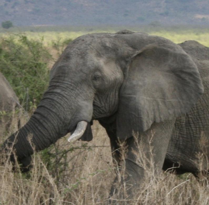
Demo 4 :: Predation
Visualizing predator-prey isoclines and dynamics
Below is a code block where the Lotka Volterra predatpr-prey system is simulated. The main plot will show the predator \(P\) (red) and prey \(N\) (blue) isoclines, as well as the starting point and trajectory of the \(P\) and \(N\) populations over time (green circle and line, respectively). On the top right inset is a plot of the two \(P\) and \(N\) population sizes plotted over time. Make sure that you understand how the isoclines determine the flow and direct how the combined trajectories of \(P\) and \(N\) (green) change over time, and how this corresponds to the population sizes shown in the inset.
Try changing the values of the parameters. Based on your derived equations for the \(P\) and \(N\) isoclines, try to anticipate what the changes you make will do to the predator/prey dynamics. One interesting thing to do: what happens when you leave all of the parameters set, but change the starting conditions?
    library(RColorBrewer)
    library(deSolve)
    pal = brewer.pal(3,'Set1')
    # Define the Rates function
    pred.flow = function(r,a,b,m,Pstart,Nstart,tmax) {
        # LV.comp = function(r1,r2,alpha,beta,K1,K2,N1start,N2start,tmax) {
        yini = c(P = Pstart,N = Nstart)

        fmap = function (t, y, parms) {
        with(as.list(y), {
            dP <- b*a*y[2]*y[1] - m*y[1]
            dN <- r*y[2] - a*y[2]*y[1]
            list(c(dP,dN))
        })
        }

        times <- seq(from = 0, to = tmax, by = 0.1)
        out   <- ode(y = yini, times = times, func = fmap, parms = NULL)

        Ptraj = out[,2];
        Ntraj = out[,3];
        timeline = out[,1];

        Pend = tail(Ptraj,n=1)
        Nend = tail(Ntraj,n=1)

        maxtraj = max(c(Ptraj,Ntraj));

        Psize = maxtraj*1.2;
        Nsize = maxtraj*1.2;

        p_isocline = m/(b*a); # = N
        n_isocline = r/a; # = P

        par(fig = c(0,1,0,1))
        plot(rep(p_isocline,100),seq(-10,Psize,length.out=100),type='l',lwd=2,col=pal[1],xlim=c(0,maxtraj*1.2),ylim = c(0,maxtraj*1.2),xlab='N population',ylab='P population',lty=2)
        lines(seq(-10,Nsize,length.out=100),rep(n_isocline,100),lwd=2,col=pal[2],lty=2)
        points(Nstart,Pstart,pch=16,cex=2,col=pal[3])
        lines(Ntraj,Ptraj,col=pal[3],lwd=2)
        points(Nend,Pend,pch=8,cex=2,col=pal[3])
        legend(0,maxtraj*1.2,c('P isocline','N isocline'),pch=16,col=pal)

        par(fig = c(0.5,1, 0.5, 1), new = T)
        plot(timeline,Ptraj,type='l',col=pal[1],xlab='Time',ylab='Pop. size',lwd=2,ylim = c(0,maxtraj))
        lines(timeline,Ntraj,type='l',col=pal[2],lwd=2,)

    }
    # Plug in parameter values and run
    pred.flow(r = 0.5, a = 0.01, b = 0.1, m = 0.1, Pstart = 70, Nstart = 100, tmax = 500)
Visualizing predator-prey isoclines and dynamics with logistic growth
The previous predator-prey model assumes that the prey grows exponentially when the predator is either absent or at low densities. What if we assume instead that the prey demonstrates (more realistic) logistic growth under these conditions, where
\[\begin{align} \frac{\rm d}{\rm dt}P &= baNP - mP \\ \frac{\rm d}{\rm dt}N &= rN \left( 1-\frac{N}{K} \right) - aNP \end{align}\]Try solving for the isoclines yourself, and confirm that you get functions that result in what is shown in the code block below. The orientation of the isoclines also suggest that flow is asymmetric from one isocline-derived quadrant to another. What is the effect of this asymmetry on the resulting dynamics? Explore similar parameter combinations as those above… how are the dynamics similar and different?
    library(RColorBrewer)
    library(deSolve)
    pal = brewer.pal(3,'Set1')
    # Define the Rates function
    pred.flow = function(r,a,b,m,K,Pstart,Nstart,tmax) {
        # LV.comp = function(r1,r2,alpha,beta,K1,K2,N1start,N2start,tmax) {
        yini = c(P = Pstart,N = Nstart)

        fmap = function (t, y, parms) {
        with(as.list(y), {
            dP <- b*a*y[2]*y[1] - m*y[1]
            dN <- r*y[2]*(1 - y[2]/K) - a*y[2]*y[1]
            list(c(dP,dN))
        })
        }

        times <- seq(from = 0, to = tmax, by = 0.1)
        out   <- ode(y = yini, times = times, func = fmap, parms = NULL)

        Ptraj = out[,2];
        Ntraj = out[,3];
        timeline = out[,1];

        Pend = tail(Ptraj,n=1)
        Nend = tail(Ntraj,n=1)

        maxtraj = max(c(Ptraj,Ntraj));

        Psize = maxtraj*1.2;
        Nsize = maxtraj*1.2;

        p_isocline = m/(b*a); # = N
        n_isocline = r/a - (r/(a*K))*seq(0,2*K,length.out=100); # = P

        par(fig = c(0,1,0,1))
        plot(rep(p_isocline,100),seq(-10,Psize,length.out=100),type='l',lwd=2,col=pal[1],xlim=c(0,maxtraj*1.2),ylim = c(0,maxtraj*1.2),xlab='N population',ylab='P population',lty=2)
        lines(seq(0,2*K,length.out=100),n_isocline,lwd=2,col=pal[2],lty=2)
        points(Nstart,Pstart,pch=16,cex=2,col=pal[3])
        lines(Ntraj,Ptraj,col=pal[3],lwd=2)
        points(Nend,Pend,pch=8,cex=2,col=pal[3])
        legend(0,maxtraj*1.2,c('P isocline','N isocline'),pch=16,col=pal)

        par(fig = c(0.5,1, 0.5, 1), new = T)
        plot(timeline,Ptraj,type='l',col=pal[1],xlab='Time',ylab='Pop. size',lwd=2,ylim = c(0,maxtraj))
        lines(timeline,Ntraj,type='l',col=pal[2],lwd=2,)

    }
    # Plug in parameter values and run
    pred.flow(r = 0.5, a = 0.01, b = 0.1, m = 0.1, K = 500, Pstart = 70, Nstart = 100, tmax = 500)
