Demo 3 :: Game Theory

< Back to Course Page

Games in Biology

We are all used to games, from Uno to World of Warcraft, if that’s your bag. But the basic idea of a game - pitting players against each other or against the board itself - captures some basic and universal ideas that are vital for understanding ecology and evolutionary biology.

In many ecological contexts, the games organisms play involve an interaction with another player. This means that the outcome of the game is conditioned on the strengths and weaknesses the other player brings to the table. For example, imagine a beetle population where there are two morphs: a smaller-sized morph and a larger-sized morph. These morphs reflect different allelic combinations at the genetic level. Because both small and large morphs are of the same species, they compete for the same types of resources. This competition can be described as a game, and the game is expected to have different outcomes depending on who is playing. For example, let’s follow an individual that is a large body-size morph. While foraging for resources, it will encounter morphs of its own larger size, as well as morphs of a smaller size. The costs and benefits of engaging with these potential competitors will influence the outcome and ultimately the individual’s fitness. As we have so often explored, fitness = survival + reproduction. If we are discussing the frequency of different alleles within a population, this means that allelic combinations that are more fit - that play games with strategies that maximize fitness - will be favored and potentially overtake the population.

The Payoff Matrix

We can visualize a simple game with a Payoff Matrix. The way we read this matrix is by considering the rows of the matrix as representing alternative player types and the columns of the matrix as describing individuals that are encountered. So take the matrix below… this describes the most famous game scenario, called The Prisoner’s Dilemma. We follow the outcome of a prisoner who is planning an escape from jail with a co-conspirator. The prisoner can take on either strategy (the rows of the matrix): they can cooperate with their co-conspirator, or they can defect and turn their co-conspirator in to the authorities. Likewise, their co-conspirator can take on the same set of strategies (the columns of the matrix). They can cooperate or they can defect.

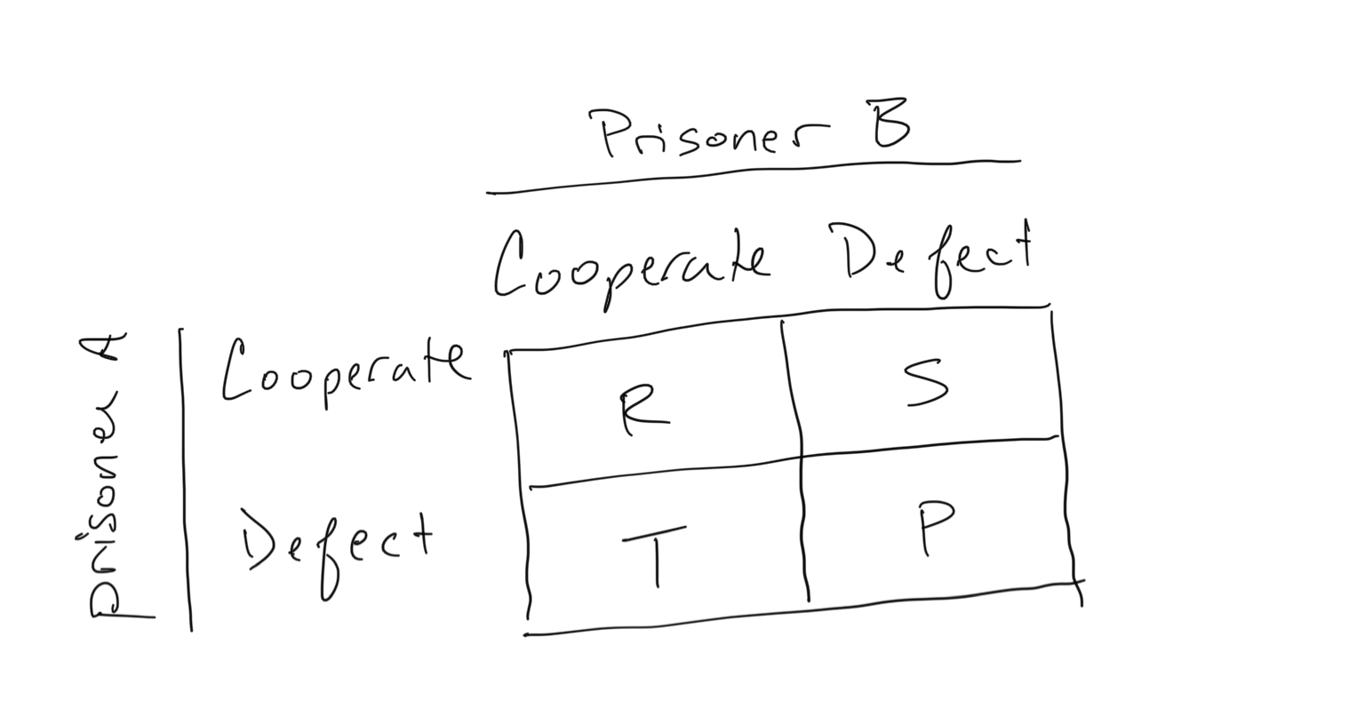
The elements of the Payoff Matrix describe what Prisoner A receives when the different scenarios outlined in the payoff matrix occur. So there are only a few things that can happen here:

1. Prisoner A (PA) cooperates and prisoner B (PB) cooperates as well. PA and PB receive \(R\), the reward (this ‘reward’ could also represent a lesser punishment)
2. PA cooperates, but PB defects. PA receives \(S\). This is the sucker’s payoff
3. PA defects, but PB cooperates. PA receives \(T\). This is the temptation payoff
   * Note that for (2) PB in that scenario receives \(T\)
   * Note that for (3) PB in that scenario receives \(S\)
   * I.e. this matrix is symmetric
4. Both prisoners defect, both receiving \(P\). This is the punishment payoff.

The question that we aim to address is: what strategy maximizes the Prisoner’s fitness? Or posed alternatively: what is the strategy that maximizes PA’s payoff? This depends on the values of \((R,S,T,P)\). How great is the reward? How bad is the sucker’s payoff? How tempting is the temptation payoff? How bad is the punishment payoff? In the classic prisoner’s dilemma, we assume that

So the temptation payoff offers the highest reward, followed by the reward both prisoners receive by cooperating, and where the sucker’s payoff offers the worst outcome.

Nash Equilibrium So what strategy is the best? We define the Nash Equilibrium as the strategy where neither player can increase their payoff by changing their strategy. In the case of the Prisoner’s Dilemma, the Nash Equilibrium is mutual defection, where both prisoner’s receive \(P\). How do we evaluate whether this strategy is a Nash Equilibrium? By assessing the change in payoff if the player switches strategy. Let’s consider two possibilities:

• If both players defect and receive \(P\), either player switching to cooperate means that it will give up \(P\) and earn instead the sucker’s payoff \(S\). Because \(P>S\), this change in strategy is worse, so Defect-Defect is at Nash Equilibrium
• If both players cooperate and receive \(R\), if one player switches its strategy to defect it will instead earn the temptation payoff \(T\), relegating the cooperating player to the sucker’s payoff \(S\). Because \(T>R\), cooperate-cooperate is not at Nash Equilibrium
• If one player defects, and the other cooperates, the defector does indeed earn a higher reward, but it cannot increase its reward by switching to cooperation. However, the other player (the cooperator) does earn a higher reward if it switched to defect. So defect-cooperate is not at Nash Equilibrium.

Discussion

1. What set of inequalities in \((R,T,S,P)\) is needed for cooperation to be at Nash Equilibrium?
2. Consider other limitations of this model. What things not included may promote cooperation?

Game theory in ecology

We are now going to take what we’ve learned from the Prisoner’s Dilemma game and leverage it to understand concepts foundational to ecology and evolutionary biology. Let’s revisit the example of a beetle population where there are two morphs: a smaller-bodied and a larger-bodied morph within a single population. As the smaller and larger morphs go out into the environment and forage for limited resources, we might assume that the potential payoffs will differ depending on who encounters whom.

• Type A = Large Morph
• Type B = Small Morph

We can construct a payoff matrix to represent the rewards obtained when one morph encounters and competes with another:

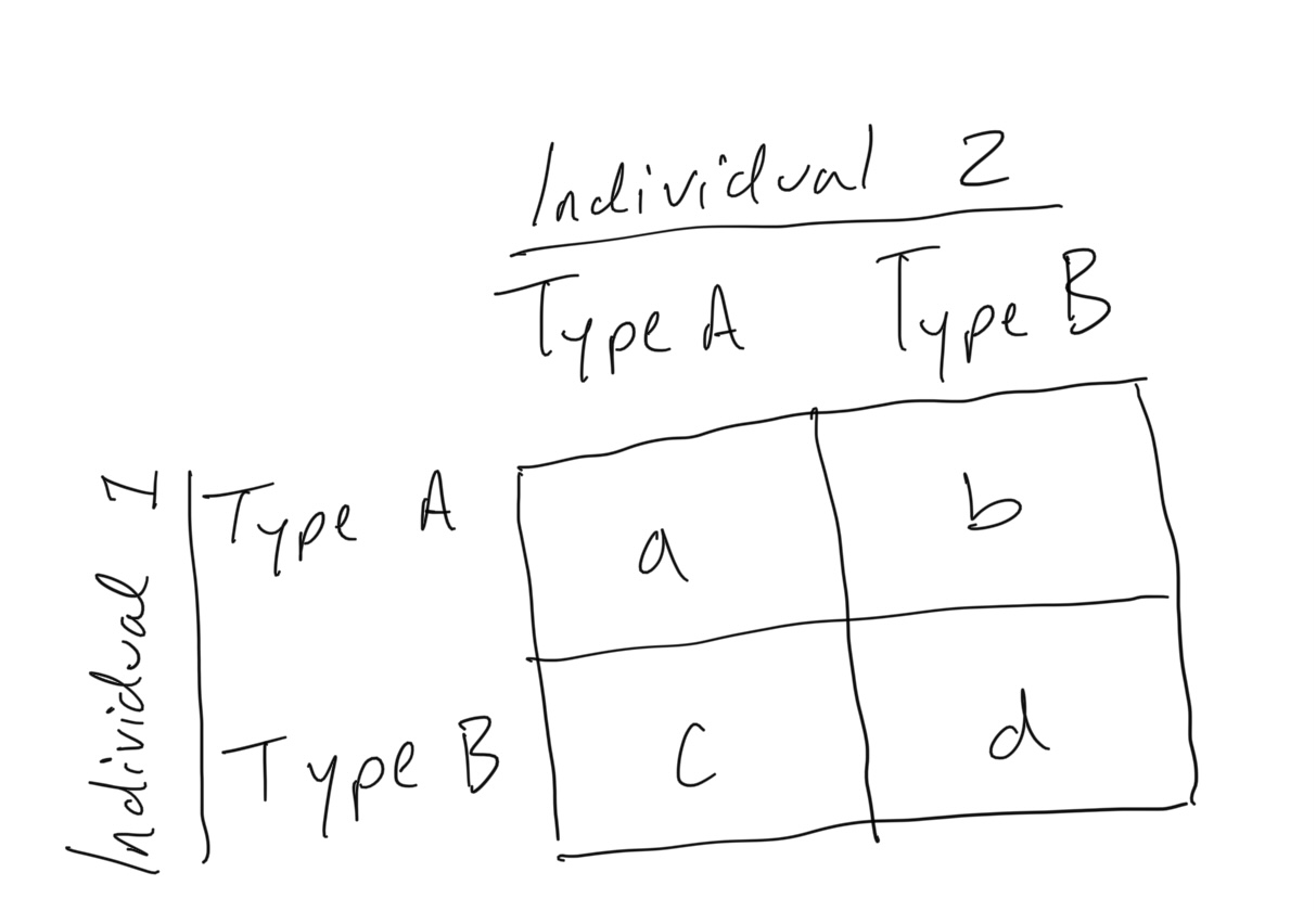
In this payoff matrix, we represent the rewards as follows:

• \(a\): The reward the A-type receives when it encounter another A-type
• \(b\): The reward the A-type receives when it encounters a B-type
• \(c\): The reward the B-type receives when it encounters an A-type
• \(d\): The reward the B-type receives when it encounters a B-type

We have not given these parameters values because we will want to explore the effects of different values in a moment. But the effects on what? How do we translate the rewards for this game to something that has ecological meaning? We now need to imagine ourselves in the ecological theater. Imagine you are a beetle foraging in the environment for a given resource, and also assume that all resources will be contested. What is the probability that you will encounter a resource contested by an A-type large morph beetle? What is the probability that you will encounter a resource contested by a B-type small morph beetle? Without additional information, we can assume that the population is evenly mixed and that our encounters with these contested resources/competitors will scale with the proportion of small- and large-morphs in the population. Moreover we will assume that the fitness accrued is directly proportional to the rewards we obtain through our encounters.

So the proportion of A-type in a population of \(N_T\) individuals is \(x = N_A/N_T\). This means that \((1-x) = N_B/N_T\). Now we can define the fitness of each:

So… if the A-type makes up most of the population, an individual of A-type is more likely to intercept and compete with an individual of A-type (thereby receiving a reward of size \(a\) with probability \(x\)), and an individual of B-type is more likely to intercept and compete with an individual of A-type (thereby receiving a reward of size \(c\) with probability \(x\)). If, by chance, an individual of A-type intercepts an individual of B-type, it will receive a reward of size \(b\) with probability \((1-x)\). Similarity, if an individual of B-type intercepts and individual of B-type, it will receive a reward of size \(d\) (with probability \((1-x)\)). The exciting thing is that this gives us useful information regarding the future of A-type individuals and B-type individuals in the population.

Discussion

1. If higher relative fitness is tied to higher relative growth rates, what will it mean for \(\Phi_A > \Phi_B\)? And for \(\Phi_B > \Phi_A\)?
2. What does this assumption of a mixed population mean? In one sense we’ve said that in a mixed population an individual’s encounter rates with each morph is proportional to the relative composition of a given morph in a population. When should this be true and when should this be false?

Now let’s graphically explore how Fitness of A-type and B-type depends on the makeup of the population \(x\). In the code-block below we have encoded the fitness values of A-type and B-type individuals as a function of the proportion of type A in the population \(x\). If \(\Phi_A > \Phi_B\), the proportion of A-type in the population will increase. This means that we will flow from left to right along the x-axis as the composition of the population becomes dominated by A-type individuals. This is represented by the the symbol >, which denotes the flow direction along the x-axis, illustrating how the makeup of the population dynamically changes in response to different payoff matrices. If \(\Phi_A < \Phi_B\), the proportion of A-type in the population will decline. This is represented by the symbol <.

For example, the following payoff matrix corresponds to a \(\Phi_A > \Phi_B\) for all values of \(x\) (let’s call this Scenario 1):

Choose values for \((a,b,c,d)\) that satisfy these conditions and see how this translates to the functions \(\Phi_A\) and \(\Phi_B\) as a function of the proportion of A-type in the population \(x\).

    # Define the evolutionary game function
    evo.game = function(a,b,c,d) {

        # Proportion of A in population
        propA = seq(0,1,0.05)
        
        # Define fitness values of A and B
        fA = a*propA + b*(1-propA)
        fB = c*propA + d*(1-propA)

        # Plot fitness values as a function of propA
        plot(propA,fA,type='l',col='blue',lwd=2,ylim=c(min(c(fA,fB)),max(c(fA,fB))),xlab='Proportion of A in population (x)',ylab='Relative fitness')
        lines(propA,fB,col='red',lwd=2) 
        legend(0.8,max(c(fA,fB)),c('A-type','B-type'),pch=15,col=c('blue','red'))

        # Add flow information
        text(0.05,(1+0.1)*min(c(fA,fB)),'Flow',cex=1.5)
        for (i in 1:length(propA)) {
            loc = i
            if (fA[loc] > fB[loc]) {
                text(propA[i],min(c(fA,fB)),'>',cex=1.5)
            } 
            if (fA[loc] < fB[loc]) {
                text(propA[i],min(c(fA,fB)),'<',cex=1.5)
            }
            if (fA[loc] == fB[loc]) {
                text(propA[i],min(c(fA,fB)),'--',cex=1.5)
            }
        }
    }

    evo.game(a = 3, b = 5, c = 2,d = 3)

Discussion

1. Now explore the following scenarios, describing what occurs in each (keep track of the values that you use as we will re-use them below)
   1. Scenario 2: \(a < c~{\rm and}~b < d\)
   2. Scenario 3: \(a > c~{\rm and}~b < d\)
   3. Scenario 4: \(a = c~{\rm and}~b = d\)
   4. Scenario 5: \(a > c~{\rm and}~b > d\)
2. As you can see from the above scenarios, the dynamics can be more complex than one morph simply overtaking the population of another morph. What conditions are required for both morphs to co-exist in a population? For the coexistence condition, what do the values of \((a,b,c,d)\) mean in terms of the A-type being the larger beetle morph and the B-type being the smaller beetle morph? I.e. relate the magnitude of the values to outcomes of the competitive interactions.
3. The condition \((a > c~{\rm and}~b < d)\) is a special condition which we refer to as being bistable. What does this say about \(x\)? Imagine a value of \(x\) immediately to the left and right of where the flows diverge. What is expected to occur under these circumstances, and what are the implications for such a system ecologically?

Fitness and population composition over time

So we have stated that higher fitness values will correlated to growth in the proportion of different morphs (or phenotypes) in the population, but now let’s be a bit more explicit about what we mean. Let’s relate the idea of fitness to the change in population composition over time. Remember that we are not talking about changes in the size of the population, but changes in the relative composition of different morphs within a single population.

Let’s formulate two rules that will help us relate relative differences in fitness to changes in population composition:

1. If the fitness of a particular morph is better than average, then the proportion of that phenotype will grow.
2. If the fitness of a particular morph is worse than average, then the proportion of that phenotype will decline. What does it mean to be better or worse than average? The average fitness is simply the mean fitness taken across individuals in the population. Because the population composition is not necessarily even, the average fitness will be weighted towards the fitness value of the more abundant morph. We can define the mean fitness of the population as

Now let’s relate this to how the the composition of A-type \((x)\) and the composition of B-type \((1-x)\) will change over time. We will use the notation \(\Delta x\) to denote the change in \(x\) per time-step.

Notice that \(\Delta x\) is positive if \(\Phi_A > \Psi\) and negative if \(\Phi_A < \Psi\). This means that the change in \(x\) will be greater than zero, or in other words the proportion of A-type in the population will increase by the amount \(\Delta x\). Similarly \(\Delta x\) is negative if \(\Phi_A < \Psi\), meaning that the proportion of \(x\) in the population will decline by the amount \(\Delta x\). And of course the same must also be true for the proportion of B-type in the population.

These are a simple set of rules, so let’s code this into a simulation, which is presented in the code-block below. As before, we need to set the values of the payoff matrix \((a,b,c,d)\), but now we also need to set:

• propA = the initial proportion of A-type in the population
• tmax = the number over time steps of which we are simulating

    game.pop = function(a,b,c,d,propA,tmax) {
        # Define fitness of A and B
        fA = a*propA + b*(1-propA)
        fB = c*propA + d*(1-propA)

        # Define average fitness
        favg = propA*fA + (1-propA)*fB

        # Empty vectors to save data
        pA = numeric(tmax)
        Favg = numeric(tmax)
        FA = numeric(tmax)
        FB = numeric(tmax)
        pA[1] = propA

        # Time simulation
        for (t in 1:(tmax-1)) {
            fA = a*pA[t] + b*(1-pA[t])
            fB = c*pA[t] + d*(1-pA[t])
            favg = pA[t]*fA + (1-pA[t])*fB
            deltaA = pA[t]*(fA - favg)
            deltaB = (1-pA[t])*(fB - favg)

            pA[t+1] = pA[t] + deltaA
            Favg[t] = favg
            FA[t] = fA
            FB[t] = fB
        }
        plot(pA,type='l',lwd=2,ylim=c(0,1),col='blue',ylab='Proportion of Type A',xlab='Time')
        lines((1-pA),type='l',lwd=2,col='red')
        legend(0.8,1,c('Prop. A','Prop. B'),pch=15,col=c('blue','red'))

    }

    game.pop(a = 3, b = 5, c = 5,d = 3, propA = 0.1, tmax = 20)

Discussion

1. Use the values that you used above to explore the dynamic consequences of Scenarios 1-5. Do they confirm your expectations?
   1. Scenario 1: \(a > c~{\rm and}~b > d\)
   2. Scenario 2: \(a < c~{\rm and}~b < d\)
   3. Scenario 3: \(a > c~{\rm and}~b < d\)
   4. Scenario 4: \(a = c~{\rm and}~b = d\)
   5. Scenario 5: \(a < c~{\rm and}~b > d\)
2. What is the effect of setting propA to a very low value? (e.g. propA = 0.0001) Consider what this might mean for invading populations.
3. Evaluate the following: game.pop(a = 4, b = 8, c = 8,d = 3, propA = 0.00001, tmax = 20) What scenario is this with respect to? What is surprising about these results? Without simulating the dynamics of A/B-type composition within the population explicitly (i.e. given the payoff matrix alone as in the example before this one), would you have been able to predict the observed dynamics?
4. Consider what the above results might mean in an environment this is subject to frequent disturbance.