Demo 2 :: Evolution by natural selection

< Back to Course Page

Natural selection is the process by which different traits exhibited by individuals within a population are selected for or against over time. Traits that benefit the individual’s fitness are selected for, and traits that reduce the individual’s fitness are selected against. Fitness is defined by an individual’s ability to survive and reproduce. Individuals with traits that either benefit its ability to survive or produce viable offspring have greater fitness compared to those with lesser abilities within a given environment. Over generational timescales, it is the individuals with these fitness-maximizing traits that become more plentiful in the population. Evolution is defined by the change in trait distributions over this generational time-span. Importantly, natural selection is something that occurs at the individual-level; because evolution is defined with respect to changing trait distributions, it is something that occurs at the population-level.

Evolution of a particular trait within a population requires

1. Heritability (the trait is passed from parents to offspring)
2. Variability in the population (different individuals have different trait values)
3. That different trait values are linked to fitness differences

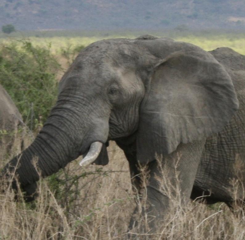
A trait can be any measurable characteristic of an individual… from anatomical or physiological characteristics such as body size or femur:tibia length ratios to the frequency of a particular behavior such as a mating vocalization. If the trait fulfills the above conditions, it is subject to selection and can evolve over time.

Trait Distributions

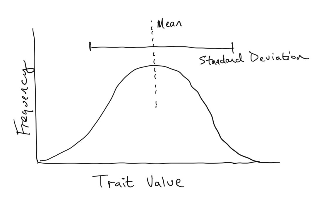
If the trait is measured as a continuous variable (say height, length, or mass), it is often normally distributed within a population. That is, the frequencies of different trait values among individuals in the population follows a normal (or Gaussian) distribution. These types of distributions can be described by two statistics: the mean and the standard deviation.

Let’s look at one of the most famous examples of natural selection that we have observed in the wild, which was documented within a population of finches on a small island in the Galapagos Archipelago.

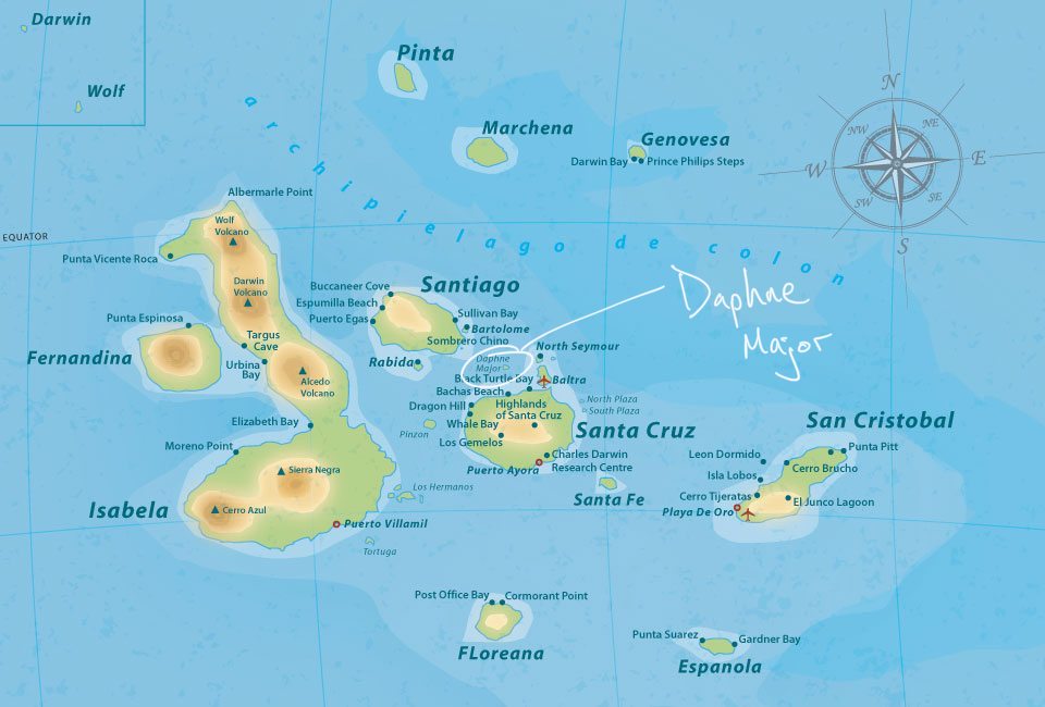
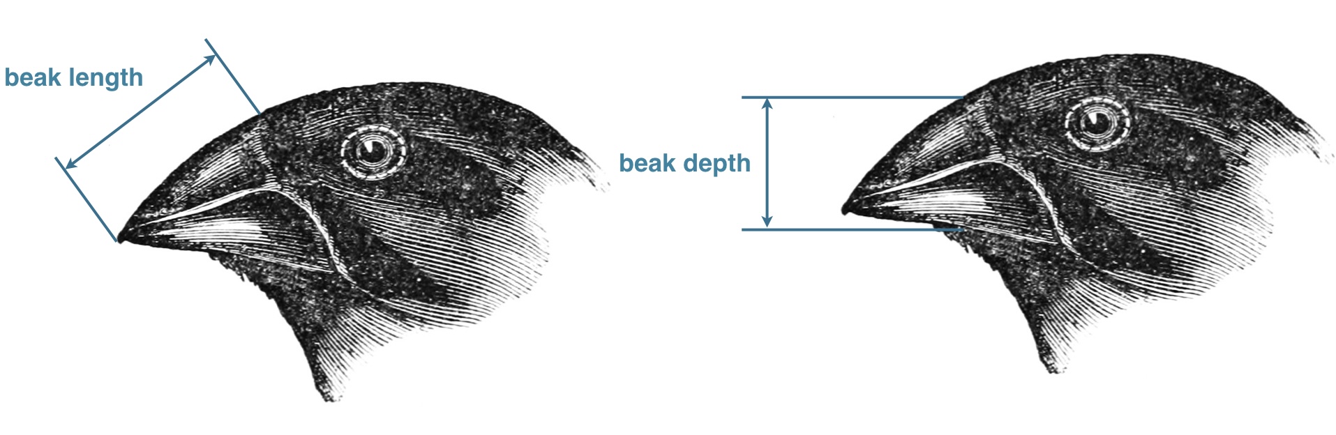
In the 1970s-80s, biologists Peter and Rosemary Grant caught and measured birds from more than 20 generations of finches on the Galapagos island of Daphne Major. In one of those years, 1977, a severe drought caused vegetation to wither, and the only remaining food source were large, tough, drought-resistant seeds, which the finches ordinarily ignored. Were the birds with larger and stronger beaks for opening these tough seeds more likely to survive that year, and did they tend to pass this characteristic to their offspring? The data are beak depths (height of the beak at its base) of 751 finches caught the year before the drought (1976) and 89 finches captured the year after the drought (1978). -Statistical Sleuth (3rd edition)

Let’s now look at the beak width data collected by Rosemary and Peter Grant on the 1976 and 1978 expedition. We will plot the frequencies of beak depth across individuals in population measured during 1976 and 1978. We will use the hist() function in R, which plots the frequency distribution. Because the number of individuals sampled in 1976 is very different (751 individuals in 1976 and 89 individuals in 1978), we have scaled the y-axis so that we are looking at the proportion of individuals with different trait values (this means the y-axis will range from \(0 \leftrightarrow 1\)).

    # We first import the Peter and Rosemary Grant data set
    library(Sleuth3)

    # Define the years as a vector
    year = ex0218$Year
    # Define the depth measures as a vector
    depth = ex0218$Depth

    # Select those measures taken in 1976
    depth_1976 = depth[which(year==1976)]

    # Select those measures taken in 1978
    depth_1978 = depth[which(year==1978)]

    # Histogram of 1976 measures (Black)
    hist(depth_1976,xlim=c(5,15),probability=TRUE,ylim=c(0,1),breaks=20,col='black',xlab='Beak depth',main='Beak depth 1976-1978',ylab='Proportion of individuals sampled')

    # Add on top histogram of 1978 measures (Gray)
    hist(depth_1978,add=TRUE,probability=TRUE,col='gray',breaks=20)

    # Legend to remind us which years the colors represent
    legend(6,0.8,c('1976','1978'),pch=15,col=c('black','gray'))

Discussion

1. Use the mean() and sd() functions to calculate the mean and standard deviation of depth measurements from 1976 (depth_1976) and 1978 (depth_1978). How does the mean and standard deviation change over time?
2. Try to explain both changes to the mean and stand deviation of the population.
3. As mentioned above, there is a large difference in the number of individuals sampled from 1976 to 1978. Why? Can we say something about the traits of the individuals who weren’t sampled in 1978? In other words, which finches were selected against and why?
4. Was this selection event caused directly or indirectly by the drought?

A Model of Evolution by Natural Selection

Recall from above that evolution is defined by the change in trait frequencies over time. In the simplest framework, this would mean that the mean of the trait distribution for the population changes over time. In this next exercise, we will examine directly how the ingredients for natural selection that are listed above are absolutely vital for evolution to take place.

Nature is complicated, and our goal now is to understand how these very particular ingredients for evolution by natural selection affect evolutionary dynamics. In order to explore these ideas, we need to strip away the complexity of the natural world to something very simple, which we call a model. We should think of this model as a toy representation of the natural world. We give this model characteristics that we hope are somewhat realistic and important to the problem that we are aiming to investigate, but without the complexities of reality to confuse our results.

So this is not a computer science class, and it isn’t important if you understand the details of the code below, but it is important that you understand what we call pseudocode. Pseudocode is what we call the collection of rules implemented by a block of code, which are generally described in the line-by-line comments.

The Pseudocode: Here is what the simulation does:

1. We imagine a population that starts with \(N_0 = 100\) individuals, each of which are given a trait value.
2. At the beginning we will randomly choose the trait value \(x\) from a normal distribution with an arbitrary mean of 0.5 and an initial standard deviation sd0 that we input.
3. At each time-step, 2 things happen:
   1. Each individual gives birth to some number of offspring. Individuals with higher trait values (values of \(x\)) have a slight reproductive advantage and give birth to more offspring. The offspring produced by an adult with a trait value \(x = m\) will have a similar trait value… we will draw the offspring’s trait from a normal distribution with a mean \(m\) and standard deviation that we call the mutation value. This describes how different the offspring is likely to be from the parent… the larger the mutation value, the more likely the offspring’s trait value will be different from the parent’s at \(x = m\). Because we are drawing the offspring’s trait from a normal distribution around \(x = m\), the offspring has an equal change of having a trait value lower than \(m\) as having a trait value higher than \(m\).
   2. Each individual has a probability of dying, regardless of its trait value.
4. We encode these rules in the code below, and keep track of the mean trait value of the population over time. Sometimes too many individuals die and the simulation stops. In the plot this is shown as the mean trait value going to zero, which just means the population is now extinct.
5. Because there are so many random things that might happen in a single simulation of a population, we want to run the simulation many times. Each repetition is independent of the others. We will plot the mean trait values of reps = 100 independently run simulations.

Now: read through the comments in the below code block, but don’t worry about the actual code itself (unless you dig that sort of thing). Copy the code block without editing anything, paste it into the R web-tool, and I’ll see you at the bottom.

    evolution.sim = function(reps,tmax,N0,sd0,mutation) {
        for (r in 1:reps) {
            # Population begins at N0 individuals
            N = N0
            # Draw random trait values for individuals from normal distribution
            # With mean of 0.5 and standard deviation given by parameter sd0
            x = rnorm(N,0.5,sd0)
            # Initialize vectors to save population and trait values
            popsize = numeric(tmax)
            meantrait = numeric(tmax)
            tic = 0
            t = 0
        
            while ((t <= tmax) && (tic == 0)) {
                # Advance time by 1
                t = t + 1
                # Reproduction
                # Roll a weighted dice
                # larger values of trait x produce more offspring
                offspring = round(rnorm(length(x),x*2,0.01),0)
                
                # Assume that offspring have same trait as parents +/- some mutation
                if (sum(offspring) >= 1) {
                    for (i in 1:length(offspring)) {
                        newx = rnorm(offspring[i],x[i],mutation)
                        x = c(x,newx)
                    }
                }

                # Mortality
                # Roll an unweighted dice
                # All individuals have the same chance of dying
                # The chance of dying increases with population size
                prob_mort = (0.6*N)/N0
                d = which(runif(length(x),0,1) < prob_mort)

                # Remove dead individual traits
                x = x[-d]

                N = length(x)
                # Save this value to a vector
                popsize[t] = N
                # Save population mean trait value to vector
                meantrait[t] = mean(x)
                
                # If population is extinct, stop
                if (length(x) <= 0) {
                    tic = 1
                }
            }
            # Plot the results
            if (r == 1) {
                plot(meantrait,type='l',lwd=2,ylim=c(0,1),col='#00000050',xlab='Time',ylab='Mean trait value of population')
            } else {
                lines(meantrait,lwd=2,col='#00000050')
            }
        }
    }

    # PARAMETERS
    # reps = number of repetitions
    # tmax = number of timesteps (keep this at 20)
    # N0 = population size at beginning (keep this at 100)
    # sd0 = trait standard deviation at beginning
    # mutation = trait standard deviation of offspring

    # RUN EVOLUTION SIMULATION
    evolution.sim(reps=100,tmax=20,N0=100,sd0=0.01,mutation=0.01)

Now that you’ve run the code, without changing any of the parameter presets, what you observe should look pretty boring. What are you looking at? You are looking at the output of the simulation described above, where we are following the traits of individuals over many generations within a population. Each line represents the mean trait value of the population over time. Because there are random, or stochastic, processes in the simulation, we are running the simulation 100 times, which accounts for the 100 lines that you observe. Any population line that jumps to zero means that that particular population has gone extinct.

Discussion

1. What is realistic and what is unrealistic about the model setup?
2. Describe the output of the simulation results
3. I mention above that the simulation results look boring, and I mean this in the sense that the mean trait value of the population does not change much over time. In other words, there is not really evolution here. Why? Pay particular attention to the sd0 and mutation values.

The effect of variation

As implied above, there is not really evolution because we have not supplied the populations variability. Variability in this model comes in two forms: a) the trait variability that we initiate the population with, and b) the variability of offspring away from the parent’s trait values. In both cases, the variability provided is very low. Oh hey… I seem to recall variation in traits being one of the 3 ingredients for evolution by natural selection to operate! Coincidence? Unlikely.

Let’s explore how increasing trait variability influences the evolutionary process. Remember we have incorporated the assumption that higher values of the trait \(x\) provides a slight reproductive advantage. In other words, individuals with larger \(x\) values have slightly more offspring than individuals with low values of \(x\).

Initial trait variability: Let’s first increase slightly the amount of variability that individuals start with at the beginning of the simulation. Try the following permutations on the original implementation of the code by replacing the last line with:

• evolution.sim(reps=100,tmax=20,N0=100,sd0=0.05,mutation=0.01)
• evolution.sim(reps=100,tmax=20,N0=100,sd0=0.1,mutation=0.01)

Discussion

1. What does the value of sd0 specify?
2. Describe what you observe as you increase sd0.
3. What do you think is the cause of this effect?

Variability of offspring from parent trait values: Now that we’ve experimented with sd0, let’s now consider the variability of the offspring away from the parent, which is encoded in the parameter mutation. If mutation=0, then the offspring has exactly the same trait as its parent. So let’s examine this first. With the previous results in mind, where sd0=0.1 and the results that you examined, let’s drop mutation=0, such that you plug in:

• evolution.sim(reps=100,tmax=20,N0=100,sd0=0.1,mutation=0)

Discussion

1. Compare these results to the case where sd0=0.1 and mutation=0.01. Are they different?
2. The big question… if there is no mutation, meaning every offspring is exactly the same as their parent, how do you explain these results???

Now let’s set the initial variability to the lower value of sd0=0.01 and explore just the impact of increasing mutation:

• evolution.sim(reps=100,tmax=20,N0=100,sd0=0.01,mutation=0.05)
• evolution.sim(reps=100,tmax=20,N0=100,sd0=0.01,mutation=0.1)

Discussion

1. Describe what you see
2. Which of the two had a larger impact on evolution? Increasing sd0 or increasing mutation?
3. Which of the two had a larger impact on the speed of evolution? In other words, the time at which some amount of change is observed?
4. What do you think the cause of these differences is?

Models tell us what questions to ask

You’ve now examined field data showcasing a selective event that resulted in evolution of a population within a very short period of time, as well as a simple model of evolution. Consider how exploration of the model, and the assumptions built into it might change our perspective when going out and studying populations in the wild. The model is useful because it is very simple in terms of the rules that we’ve injected into it, and the results that it produces may lead us to examine nature in different ways. The model is not designed to replicate nature… it is meant to capture a hypothesis of how a very few set of rules may influence how nature works. It shows us where to look. By building our assumptions into a model and understanding its output, we can go back to the island of Daphne Major and investigate whether nature actually works the way the model predicts. If we find that it does not, we have left something important out of the model, and we need to go back to the drawing board. If we find that nature works similar to model predictions, that is evidence that the relationships we have encoded into the model capture an important natural mechanism! We pat ourselves on the back and enjoy a cold beverage.

Discussion

1. What does the model suggest is important for evolution by natural selection?
2. Relate these concepts to what is observed on Daphne Major. What might you measure and investigate if you could go back to the island, now that you have model predictions to guide your thinking?
3. Challenge Round This model is very tweakable, though tweaking it will often break it (that is okay - you can’t make an omelette without breaking some eggs). How would we introduce an influence of trait \(x\) on mortality? Currently all individuals have equal probability of dying, and this probability increases as the population grows. Alter the Pseudocode above to incorporate some effect of trait \(x\) on mortality. If you are feeling daring, feel free to try to alter the code to implement your idea.
4. Insanity Round As we have explored, a reproductive advantage leads to directional selection towards higher mean trait values of \(x\). Building upon the Challenge Round idea, what if the trait-dependent mortality was disruptive? What would that mean and how would it be implemented? What would be the effect of a) directional selection via a reproductive advantage to higher values of trait \(x\) coupled with b) disruptive selection via trait-dependent mortality?