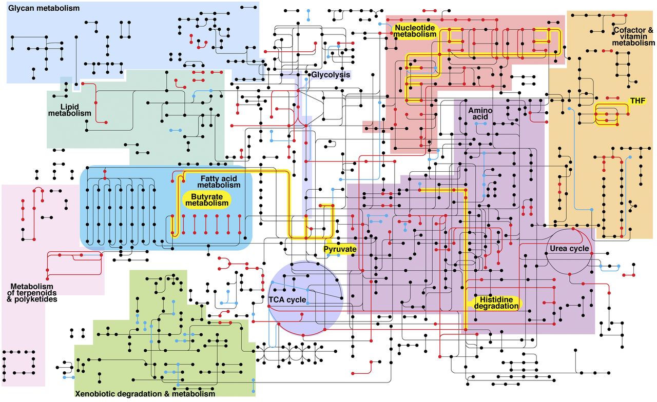
In the last section (Section 1), we investigated the role of temperature in driving and constraining organismal activity rates. But why do organisms care what the temperature is? To answer this we must consider what an organism made of. Fundamentally an organism is an incredibly complex network of chemical reactions designed to pass information into subsequent individuals (their own complex network of interactions) across generations. We call an operational unit of this complex system a metabolic network. If you have taken Introductory Biology, you have explored many of the fundamental biochemical reactions that form the basis of metabolism, including the Krebs cycle and - for photosynthetic organisms - photosynthesis. What does this metabolic network look like? Check it out:
If it looks complicated, that’s because it is. Don’t worry - this isn’t a biochemistry course, so we will turn our focus now to how this process as a whole impacts organismal ecology.
What is metabolism?
The entire metabolic process as shown above captures the energetic expenditure of what it takes to ‘run’ an organism’s physiological processes. Metabolism is thus the sum of the processes depicted above, integrated over a period of time. Metabolism fuels physiology, and physiology impacts behavior. For example, depending on the species, an individual can only pack on so much body fat. This body fat is used in part as an energy reserve - like the gas tank in your car. As it functions and interacts with the external environment, its body takes calories in via food, and burns what it doesn’t intake from fat. Excess intake gets added to fat stores. If an individual is unable to find food, fat is catabolized to fuel metabolic processes. Organisms with higher metabolic requirements must burn more energy, and this impacts how/when an individual forages for food, interacts with other individuals, reproduces, etc… the stuff of ecology. Warm-blooded organisms (endotherms) maintain a constant internal body temperature, which costs additional energy, and this affects all aspects of their lives… they must forage more frequently, they can’t go as long without food (in comparison, some snakes, which are ectotherms, can go a month or more without feeding), and reproduction is generally riskier because it is more energetically expensive.
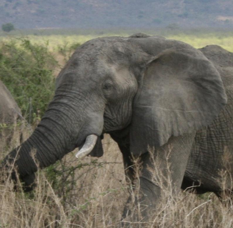
Now that we have a sense of what metabolism is, and that it has a direct impact on organismal ecology, let’s examine how metabolic rates vary species by species. We will first examine metabolic rates for mammals. Because mammals are endotherms, their metabolic rates are not expected to fluctuate with temperature as they would for ectotherms. Moreover, let us compare the metabolism of organisms across a range of body sizes… from a mouse to an elephant. But first a few items to think about.
Discussion
What relationship would you expect between metabolic expenditure and species’ body size?
What relationship would you expect if you took out the effect of body size? In other words, if you compared the metabolic expenditure of a gram of mouse to a gram of elephant?
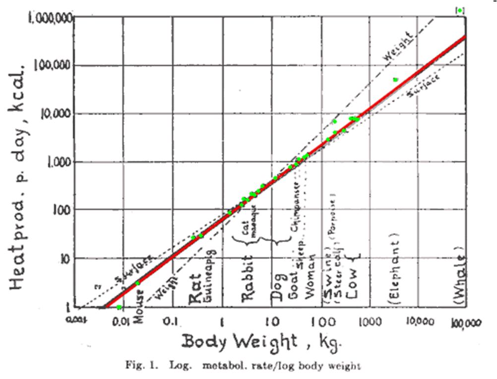
Now let’s look at one of the most famous biological relationships… the depiction of metabolic rate, measured as heat produced per day in kilocalories, as a function of species’ body mass (kg), known as the Kleiber Law
The Kleiber Curve, showing (in log-log space) the relationship between metabolic rate and body mass.
This is a figure created by Max Kleiber, a physiologist who, in the 1930s, discovered that metabolic rate scales in a very particular way with organismal body size. First, notice that the scales of the x- and y-axis are log-scaled… meaning that each successive quadrant (moving along the x- or y-axis) is 10x the size of the previous quadrant. Perhaps unsurprisingly, we observe that an elephant or whale generates more heat per day than a mouse or guineapig. With this log-spacing, the metabolic rate of species is linearly scaled with body mass.
Linear to log-log spacing refresher
As a quick refresher, what does it mean when we look at a log-log plot?
Let’s take the following curve:
\[\begin{equation}
y = a M^b
\end{equation}\]
Now, this is a curve if \(b \neq 1\). However if we take the log of both sides of this equation, we get
First, notice that because \(a\) is just a number, \(\log(a)\) is just a number. Second, this logged equation is in the standard format of a line, with a y-intercept and slope. So when we view a straight line in log-log space of the above equation, unless the slope \(b = 1\), we know it is a curved line in linear spacing.
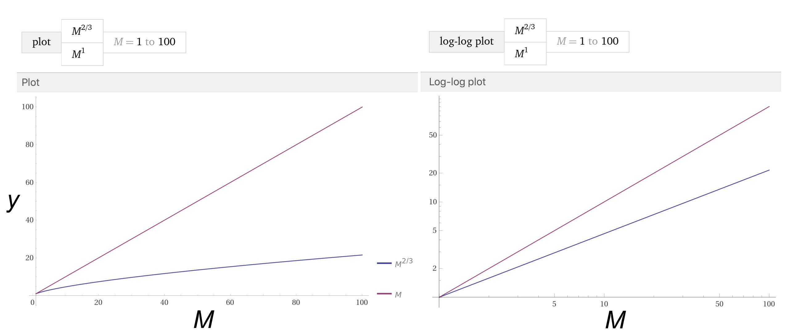
On the left is the \( y = M^1 \) (purple) and \( y = M^{2/3} \) (blue) line in linear space. Note that \( y = M^1 \) is a straight line with a 1:1 slope, whereas \( y = M^{2/3} \) is slightly curved, or nonlinear. On the right are the same lines, but in log-log space. Here, the same relationships are displayed as straight lines, as expected from the above equations. An alternative to the plot on the right is to log the relationship first, and plot it in linear space.If we did this, we would need to label the axes Log(M) and Log(y)
Now let’s play with some data of our own… Below we will experiment with plotting
# Species namessp=c('dove','fe_rat','ml_rat','pigeon','hen','fe_dog','ml_dog','sheep','woman','man','cow','steer','steer')# Species massesmass=c(0.150,0.173,0.226,0.300,1.96,11.6,15.5,45.6,56.5,64.1,388,342,679)# Species metabolic rates in Calories per hourcalperhr=c(19.5,20.2,25.5,30.8,106,443,525,1219.9,1349,1632,6421,6255,8274)# Plot the data (linear axes)plot(mass,calperhr,xlab='Mass (linear spacing)',ylab='Metabolic rate (linear spacing)')# Plot the data (log-log axes)plot(mass,calperhr,log='xy',xlab='Species Body Mass (log spacing)',ylab='Metabolic rate (log spacing)')
Discussion
What is the difference between these two figures? Relate the linear-spacing and log-spacing plots to the figure above. Do you see how the points in linear-spacing are slightly curved and that the points in log-space follow a straight line?
If we assume that the data follow \(B = a M^b\) where B is metabolic rate and M is mass (as is often standard), do you think that \(b = 1\)? How can you tell from looking at the linear- and log-spaced plots?
Origins of metabolic scaling
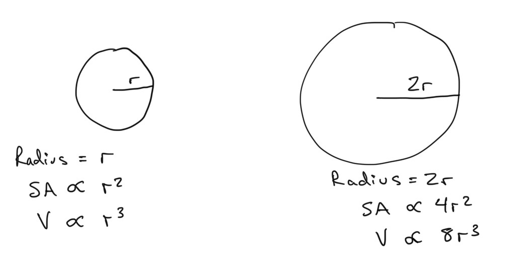
Why would metabolic rate \(B\) be expected to scale with body mass \(M\), and what scaling would be expected? (Remember - when we are discussing types of scaling, we are really talking about the value of \(b\) in the equation for metabolic rate \(B = a M^b\). We know that when this is logged, it is the value of the slope of the relationship between metabolic rate \(B\) and body mass \(M\). The parameter \(a\) just determines the intercept, which in log-log space is \(log(a)\). A linear scaling is when \(b = 1\). A superlinear scaling is when \(b > 1\), and a sublinear scaling is when \(b < 1\)). Let’s see if we can build some intuition about what to expect. There are two things to keep in mind… if we imagine a spherical organism increasing in size, the surface area and volume of a sphere scale differently:
Left: a spherical animal with radius \( r \). Right: a sperical animal with radius \( 2r \) .
where \(\propto\) means ‘in proportion to’. This way, we don’t have to write the full equation for the surface area of a sphere, which is \(SA = 4\pi r^2\), as the \(4 \pi\) is a constant and the bit we care about is that SA is in proportion to \(r^2\).
The HEAT produced by metabolism is produced in proportion to an organism’s volume (because the number of cells is in proportion to volume and each cell produces heat). However the heat must be DISSIPATED across the organism’s surface area. So the energy produced by metabolism \(B\) might be hypothesized to be scaled with volume \(V\)
BUT we know this wouldn’t work because the organism wouldn’t be able to dissipate metabolic energy as heat, which would cause it to messily explode. We are using the label \(B_{\rm geometry}\) to note the fact that we are building a relationship for \(B\) (metabolic rate) based on geometric arguments.
So \(B_{\rm geometry}\) must be tuned down so that the energy produced by the organism’s volume can be dissipated as heat across its surface. How much should it be tuned down? We can make a geometric argument for this… if the energy produced from metabolism is cubed (as is the volume), but it needs to be dissipated across the organism’s surface area, we need to tune the cubic relationship down to a squared relationship. So we need to change the exponent 3 to an exponent 2. We can do this by including an exponential term of 2/3, which converts a volumetric measure to an area measure.
\[\begin{equation}
SA \propto V^{2/3} \propto (r^3)^{2/3} \propto r^2.
\end{equation}\]
Now an individual’s body mass \(M\) is a volumetric measure. So we can suppose that metabolic rate \(B_{\rm geometry}\) should be proportional to mass tuned down by an exponent of 2/3, or
where the 2/3 exponent is how much we need to tune down the metabolic rate so that the organism avoids overheating and grossly exploding. That the heat produced by our volume needs to be tuned down in such a way that it can be gotten rid of across our surface area is a necessary limitation of being a 3-Dimensional organism.
The question is: is this correct? Let’s plot a line through our data that increases \(\propto M^{2/3}\). We will use a y-intercept value that fits the data reasonably well.
# Species namessp=c('dove','fe_rat','ml_rat','pigeon','hen','fe_dog','ml_dog','sheep','woman','man','cow','steer','steer')# Species massesmass=c(0.150,0.173,0.226,0.300,1.96,11.6,15.5,45.6,56.5,64.1,388,342,679)# Species metabolic rates in Calories per hourcalperhr=c(19.5,20.2,25.5,30.8,106,443,525,1219.9,1349,1632,6421,6255,8274)# Plot the data (with log-log axes but not explicit in the axes title)plot(mass,calperhr,log='xy',xlab='Species Body Mass',ylab='Metabolic rate')# Plot the 2/3 scaling line (stippled)lines(mass,exp(4.29)*mass^(2/3),lwd=2,lty=2)
Discussion
Does the 2/3 line match the data well?
Are there certain species for which it does and does not match well?
Cheating 3-Dimensional limitations with Fractal Branching
We’ve spent the last few minutes convincing ourselves that a 2/3 scaling is a reasonable expectation based on the geometry of 3-Dimensional organisms. Now we will see that this is wrong, and that there is a better solution than a 2/3 scaling, even though 2/3 would seem to be a strict limitation of being a 3-Dimensional organism in a 3-Dimensional environment.
First, let’s think about why it might be beneficial for an organism’s metabolism to scale differently than the 2/3 limitation. Because 2/3-scaling is less than a 1:1 scaling, the metabolism of larger organisms is lower - per unit biomass - than a smaller organism. So if we think of a cubic gram of mouse vs. a cubic gram of elephant, the cubic gram of mouse is generating more energy. If metabolic scaling can be pushed >2/3, the energy produced per unit biomass is elevated, thereby increasing the energetic ‘bank account’ of an organism, especially those of larger body size.
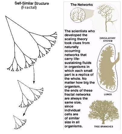
Fractal Branching Life has found a way to cheat the limitations of 3-Dimensions, which is mind-blowing. On the left you can see a depiction of branching alveoli, which function to distribute gases between the air we inhale/exhale to/from blood vessels within the lungs. Our body is filled with these distribution channels - from alveoli to blood capillaries - that are organized in fractal branching patterns. The argument we made for the 2/3 scaling is based on the dissipation of heat from a 3-D volume to a 2-D surface. The reasoning behind a 3/4 scaling is that the primary limitation is the DISTRIBUTION of materials (nutrients, gasses, waste) throughout our bodies, all of which is facilitated by distribution channels that exhibit fractal branching geometries. Strangely, these fractal shapes have a dimensionality closer to 4-Dimensions rather than 3-Dimensions 🤯. The mechanisms themselves are complex, and involve advanced mathematical and physical reasoning. If you dig that kind of thing, check out this paper. The following video does a nice job discussing this near-4-Dimensional geometry, so check it out before or after section. (Note: the paper is optional but you are expected to watch the video!)
For now, let’s look at that plot again, but by fitting a 3/4 power law line in addition to the 2/3 power law line. We will keep the line for the 2/3 power law stippled, and the line for the 3/4 power law solid. Which fits better?
# Species namessp=c('dove','fe_rat','ml_rat','pigeon','hen','fe_dog','ml_dog','sheep','woman','man','cow','steer','steer')# Species massesmass=c(0.150,0.173,0.226,0.300,1.96,11.6,15.5,45.6,56.5,64.1,388,342,679)# Species metabolic rates in Calories per hourcalperhr=c(19.5,20.2,25.5,30.8,106,443,525,1219.9,1349,1632,6421,6255,8274)# Plot the dataplot(mass,calperhr,log='xy',xlab='Species Body Mass',ylab='Metabolic rate')# Plot the 2/3 scaling line (stippled)lines(mass,exp(4.29)*mass^(2/3),lwd=2,lty=2)# Plot the 3/4 scaling line (solid)lines(mass,exp(4.29)*mass^(3/4),lwd=2)
Discussion
How does cheating the 3-D limitations of nature benefit organisms? In other words, what are the consequences of having a 3/4 scaling law rather than a 2/3 scaling law?
What other natural things (living or nonliving) exhibit fractal branching patterns?
Mammalian population densities
If we go out in nature and begin measuring things, it is often surprising how many qualities of ecological systems exhibit scaling relationships that appear to relate, and sometimes be the same as, the 3/4 power law. While the 3/4 power law for metabolism has some very well-defined theory that may explain the underlying mechanism, many other power-scale ecological relationships remain mysterious. Importantly, these scaling relationships are usually only evident when we look across many species and many ecosystems…
For example, let’s look at the population densities of different mammal species, since we will be focusing so much on populations this semester. A population densities is generally defined by number of individuals within a given area… for example, we might count 3 antelope within a hectare or 1 mouse per 10 meters square. When comparing densities it is thus necessary to hold constant the area (the denominator). So if our area is a square meter, a habitat might hold 5 crickets/square meter, 0.1 antelopes/square meter (i.e. 1 per 10 square meters), or 0.001 elephants per square meters (i.e. 1 per 1000 square meters). Let’s look at some data.
# Enter Species Body Massmass=c(7250,6550,7250,960,6000,6000,1070,680,1200,241,2520,2600,2600,8000,6000,4050,3550,3600,3500,4500,4350,4950,2700,177,8150,9850,9500,7800,300,260,127000,5900,5800,5800,6100,12500,600,2700,2100,1700,5000,7850,9100,5150,385,725,1250,22700,45000,19500,17500,13900,19500,18600,1150,425,1024,53000,6250,12800,8350,8150,6300,8350,6300,8150,3600,315,600,665,665,10700,17100,83400,52400,158000,403000,31000,31800,46500,29800,48100,31000,551000,850000,125000,263000,568000,149000,274000,75000,1e+05,21700,14000,12500,310000,175000,170000,138000,203000,70000,122000,58800,21000,912000,225000,197000,13300,211000,194000,90600,69300,89000,42000,4940,20000,14200,89300,85100,14300,167000,13600,250000,75900,24000,60900,65700,1e+05,12300,8210,59400,28000,43500,42500,55300,11300,544000,453000,21700,90600,110000,40800,74800,171000,3200,47500,2220000,952000,1120000,259000,390000,270000,1255000,997000,3e+05,175000,1810000,2860000,2430,1360,2420,3030,2710,3020,3400,154,1640,854,692,1130,1020,22,146,42,8200,29.1,127,20,36,33,70,103,143,71,7,22.5,257,170,210,40,40,40,487,1020,222,27,23,31,28,4000,30.5,68.7,241,400,1130,88,2700,2000,5,13.5,8.2,55,56,60,108,145,72,38.5,65,53,145,475,400,35,8620,39,97,26,69,69,65,63,32800,44.5,30,81,54,65,44,39,400,64,3400,3950,65,116,250,36,27,71,47,35,43,35,49,49,8.6,6.4,8.5,11.8,108,34,17.8,254,250,248,130,260,21,218,86,65,49,42,35,40,30,76.5,24.1,40,59,40,50,136,121,112,7.4,17,7.5,20,15,28,42,23,35,21,20,15,24,52,39,44,53,50,38,316,800,70,72,62,125,321,122,112,251,54,85,21,16,44,115,45,530,275,680,275,120,129,50,350,500,351,107,200,800,71,100,27,200,97,207,101,51,62,42,154,93,34,18,29,56,118000,2700,3500,300,25000,12000,31900,41400,11000,1360,872,1250,3000,2800,2080,22500,10000,17.8,3.8,10.6,33.4,55,805,9.3,8,4.2,4.5,5.3,7,18.5,5.3,76,134,210,220,25,51.4,45,25.4,50,64,27.1,70.9,23.8,85,253,51,1800,10900,2404,105000,1430,9070,3750,8000,595,3250,2800,3500,20000,4000,35,560,80,45,40,15,338,5700,50000,5500,1020,5440,12500,14000,45600,10000,65000,9500,16000,6500,5000,59500,85500,13600,4380,7480,1800,4800,820,1780,525,3700,5000,20700,10200,28600,883,3250,670,78.9,80,150000,41400,130000,71700,8620,386000,5440,8160,2490,10700,7050,153000,233000,1070)# Enter Species population densitiesdensity=c(2.5,5.1,7.4,10,1.35,4.5,15,25.5,1.5,90,3.7,8,3.5,3.3,4.5,5.3,10.8,2,2,4.2,3.4,2.25,2.25,25,23,11.2,3,0.03,1.75,1.75,0.18,0.51,3,0.62,2.2,1.2,28.8,25,103,35,2.5,3.5,2,10,12.1,21.5,2.62,0.4,0.25,1.03,0.4,0.18,1.25,0.23,0.9,67.5,4,0.2,2.9,5.7,15,10.7,4.2,3.3,1.14,15.4,17.5,3.3,2.3,2.5,2.5,0.52,6.95,0.776,1.31,0.206,0.072,0.083,0.465,0.093,0.48,1.3,3.5,0.032,0.1,0.0146,0.085,0.061,0.27,0.12,0.31,0.46,0.86,0.8,0.4,0.093,0.548,1.27,0.142,0.759,1.88,1.1,0.106,0.664,0.0937,0.0774,0.066,1.79,0.911,0.169,1.55,0.015,0.051,0.103,11.1,1,0.353,1,1.26,0.46,0.075,0.19,0.036,0.168,0.571,0.13,0.027,0.288,0.06,0.085,0.146,0.669,0.081,0.08,0.284,0.153,0.381,0.0345,0.746,0.0209,0.0182,1.03,11,0.179,0.31,0.35,0.074,0.084,0.0093,0.374,0.257,0.15,0.627,0.012,0.063,0.08,0.049,0.109,2.56,14.1,1.3,0.997,10.1,1.86,0.584,55.8,13.1,3.54,54.4,58.8,6.88,345,159,330,2.5,362.6,3.2,124,94.9,255,1240,86.2,3090,25.7,155,40,2.1,0.65,11.1,40,135,28.6,204,27.8,125,116,189,55.6,460,4.03,25,74.1,24.7,420,247,194,9,10,98.5,198,117,142.9,58.5,50.4,46.9,145,95,120.9,131,44.9,20.5,0.7,4,161,0.39,170,53.1,195,29.3,109,69.5,9.1,10.4,32.5,66.6,290,38.7,77.7,138,62,17.5,25.6,29.6,61.6,66.7,15,239,220,377,1990,750,300,675,1200,450,404,38,86.8,69.9,91.9,18.9,317,3.1,988,14,9.3,161,160,35.1,1400,422,230,5.02,53.2,12.9,105,62,5.88,245.5,20,190,170,10,297,270,111,29.4,48,21.4,297,70.1,58.5,479,29.3,465,189,106,104,445,409,43.4,26.3,87.6,77.7,190,106,58.3,7.9,2.7,448,177,3.8,365,22.7,335,5,6.9,59.8,153,22.4,14.4,87,70.1,4.5,43.1,30,146,222,5,513,50,328,10.5,31.8,33,9.4,2.3,185,382.2,206,14.8,72.5,52.8,55,34.3,220,248,21.4,643,33,27.9,0.0121,40.7,19,15,2.08,4.7,1.5,0.07,10,1.96,12.5,8.3,51.1,15,7.5,1.1,2,62.1,15.3,39.2,8.17,140,60,104.6,56.4,120.7,6.9,62.1,71.7,94.9,110.3,104.5,7.4,0.7,5.9,867,381.5,20,202,161,31.9,4.5,29.7,29.4,62,1.08,6.9,1.075,0.282,0.85,0.029,1.81,0.16,0.188,0.075,0.5,0.69,5,1.33,0.018,0.6,168.9,1.98,5.1,6.3,18,5,10.5,1.16,0.00601,0.0175,0.22,0.023,0.0258,0.0296,0.002,0.2,0.0506,0.1,0.0625,0.4,0.2,0.002,0.001,0.025,0.0414,0.073,0.385,0.24,0.6,0.213,0.15,0.193,0.5,0.0022,0.013,0.0043,0.12,0.0235,0.82,1.053,3.6,0.013,0.021,0.0056,0.0012,0.22,0.00162,0.16,0.226,1.44,0.34,0.71,0.0818,0.0129,6.9)/100000# Plot the data# Note here we are logging the data before plotting, so# values will be log() of the original data entered aboveplot(log(mass),log(density),xlab='Log Species Body Mass (g)',ylab='Log Population Density (Individuals/Meter^2)',pch=16)# Find the best linear fit to the logged-data# This means we are looking for the line that best passes through the logged data# We are fitting the line through the logged data because we know that these # relationships in log-log spaces are simple linesm=lm(log(density)~log(mass))# This prints the best-fit line on top of our dataabline(m)# What is the slope of this line? Print it out!slope=m$coefficients[2]print(paste("Slope of Data = ",slope))
Discussion
Before looking at the best-fit line, what is the general nature of the data… what does this mean for populations of smaller vs. larger organisms?
Without any other information, can we use this perspective to gain insight into the extinction risk of larger organisms? Would you expect larger organisms to be at greater or lesser risk of extinction?
What is the slope of the best-fit line? Any similarities to the 3/4 scaling law?
The Energy Equivalence Hypothesis
Now we will attempt to combine the ideas behind metabolic rates and observations of mammalian population densities to attempt to achieve insight into the workings of natural ecosystems. Let’s imagine individuals and the populations within which they live as little factories producing an energetic output. In a sense, this perspective is not inaccurate. Species are factories that convert energy from the outside into their own biomass, and pass down this biomass in the form of reproduction… over and over and over. How much energy does an individual produce per unit time? Well, we have this relationship in the form of \(B = aM^{3/4}\), where \(a\) determine the y-intercept (and varies depending on units). Here we will use \(a = 0.047\) (with units of Watt grams\({}^{-3/4}\), but the main thing you need to know is that this is a unit of produced energy).
From above we have, for a species of body mass \(M\), an expectation for the population density (individuals/area). And from the relationship for metabolic rate as a function of body mass, we have the energy processed by a species of a given body mass \(M\). ***If we multiply the amount of energy used by an individual by the number of individuals in an area, we can calculate the amount of energy required by species populations as a function of their body mass! We can do this by simply multiplying together their expected metabolic rates by their population densities:
where \(N\) is the number of individuals of that species within a given area, or the species’ population density. To clarify, this isn’t the energy produced for the entire population… it’s the energy produced for a given population within a particular area. Denser populations mean that there are more individuals in that area, sparser populations mean that there are fewer individuals in that area. See the above plot to observe how these population densities change with species body size.
Now let’s calculate the amount of energy used within a given area for populations of mammalian species as a function of body mass!
# Enter Species Body Massmass=c(7250,6550,7250,960,6000,6000,1070,680,1200,241,2520,2600,2600,8000,6000,4050,3550,3600,3500,4500,4350,4950,2700,177,8150,9850,9500,7800,300,260,127000,5900,5800,5800,6100,12500,600,2700,2100,1700,5000,7850,9100,5150,385,725,1250,22700,45000,19500,17500,13900,19500,18600,1150,425,1024,53000,6250,12800,8350,8150,6300,8350,6300,8150,3600,315,600,665,665,10700,17100,83400,52400,158000,403000,31000,31800,46500,29800,48100,31000,551000,850000,125000,263000,568000,149000,274000,75000,1e+05,21700,14000,12500,310000,175000,170000,138000,203000,70000,122000,58800,21000,912000,225000,197000,13300,211000,194000,90600,69300,89000,42000,4940,20000,14200,89300,85100,14300,167000,13600,250000,75900,24000,60900,65700,1e+05,12300,8210,59400,28000,43500,42500,55300,11300,544000,453000,21700,90600,110000,40800,74800,171000,3200,47500,2220000,952000,1120000,259000,390000,270000,1255000,997000,3e+05,175000,1810000,2860000,2430,1360,2420,3030,2710,3020,3400,154,1640,854,692,1130,1020,22,146,42,8200,29.1,127,20,36,33,70,103,143,71,7,22.5,257,170,210,40,40,40,487,1020,222,27,23,31,28,4000,30.5,68.7,241,400,1130,88,2700,2000,5,13.5,8.2,55,56,60,108,145,72,38.5,65,53,145,475,400,35,8620,39,97,26,69,69,65,63,32800,44.5,30,81,54,65,44,39,400,64,3400,3950,65,116,250,36,27,71,47,35,43,35,49,49,8.6,6.4,8.5,11.8,108,34,17.8,254,250,248,130,260,21,218,86,65,49,42,35,40,30,76.5,24.1,40,59,40,50,136,121,112,7.4,17,7.5,20,15,28,42,23,35,21,20,15,24,52,39,44,53,50,38,316,800,70,72,62,125,321,122,112,251,54,85,21,16,44,115,45,530,275,680,275,120,129,50,350,500,351,107,200,800,71,100,27,200,97,207,101,51,62,42,154,93,34,18,29,56,118000,2700,3500,300,25000,12000,31900,41400,11000,1360,872,1250,3000,2800,2080,22500,10000,17.8,3.8,10.6,33.4,55,805,9.3,8,4.2,4.5,5.3,7,18.5,5.3,76,134,210,220,25,51.4,45,25.4,50,64,27.1,70.9,23.8,85,253,51,1800,10900,2404,105000,1430,9070,3750,8000,595,3250,2800,3500,20000,4000,35,560,80,45,40,15,338,5700,50000,5500,1020,5440,12500,14000,45600,10000,65000,9500,16000,6500,5000,59500,85500,13600,4380,7480,1800,4800,820,1780,525,3700,5000,20700,10200,28600,883,3250,670,78.9,80,150000,41400,130000,71700,8620,386000,5440,8160,2490,10700,7050,153000,233000,1070)# Enter Species population densitiesdensity=c(2.5,5.1,7.4,10,1.35,4.5,15,25.5,1.5,90,3.7,8,3.5,3.3,4.5,5.3,10.8,2,2,4.2,3.4,2.25,2.25,25,23,11.2,3,0.03,1.75,1.75,0.18,0.51,3,0.62,2.2,1.2,28.8,25,103,35,2.5,3.5,2,10,12.1,21.5,2.62,0.4,0.25,1.03,0.4,0.18,1.25,0.23,0.9,67.5,4,0.2,2.9,5.7,15,10.7,4.2,3.3,1.14,15.4,17.5,3.3,2.3,2.5,2.5,0.52,6.95,0.776,1.31,0.206,0.072,0.083,0.465,0.093,0.48,1.3,3.5,0.032,0.1,0.0146,0.085,0.061,0.27,0.12,0.31,0.46,0.86,0.8,0.4,0.093,0.548,1.27,0.142,0.759,1.88,1.1,0.106,0.664,0.0937,0.0774,0.066,1.79,0.911,0.169,1.55,0.015,0.051,0.103,11.1,1,0.353,1,1.26,0.46,0.075,0.19,0.036,0.168,0.571,0.13,0.027,0.288,0.06,0.085,0.146,0.669,0.081,0.08,0.284,0.153,0.381,0.0345,0.746,0.0209,0.0182,1.03,11,0.179,0.31,0.35,0.074,0.084,0.0093,0.374,0.257,0.15,0.627,0.012,0.063,0.08,0.049,0.109,2.56,14.1,1.3,0.997,10.1,1.86,0.584,55.8,13.1,3.54,54.4,58.8,6.88,345,159,330,2.5,362.6,3.2,124,94.9,255,1240,86.2,3090,25.7,155,40,2.1,0.65,11.1,40,135,28.6,204,27.8,125,116,189,55.6,460,4.03,25,74.1,24.7,420,247,194,9,10,98.5,198,117,142.9,58.5,50.4,46.9,145,95,120.9,131,44.9,20.5,0.7,4,161,0.39,170,53.1,195,29.3,109,69.5,9.1,10.4,32.5,66.6,290,38.7,77.7,138,62,17.5,25.6,29.6,61.6,66.7,15,239,220,377,1990,750,300,675,1200,450,404,38,86.8,69.9,91.9,18.9,317,3.1,988,14,9.3,161,160,35.1,1400,422,230,5.02,53.2,12.9,105,62,5.88,245.5,20,190,170,10,297,270,111,29.4,48,21.4,297,70.1,58.5,479,29.3,465,189,106,104,445,409,43.4,26.3,87.6,77.7,190,106,58.3,7.9,2.7,448,177,3.8,365,22.7,335,5,6.9,59.8,153,22.4,14.4,87,70.1,4.5,43.1,30,146,222,5,513,50,328,10.5,31.8,33,9.4,2.3,185,382.2,206,14.8,72.5,52.8,55,34.3,220,248,21.4,643,33,27.9,0.0121,40.7,19,15,2.08,4.7,1.5,0.07,10,1.96,12.5,8.3,51.1,15,7.5,1.1,2,62.1,15.3,39.2,8.17,140,60,104.6,56.4,120.7,6.9,62.1,71.7,94.9,110.3,104.5,7.4,0.7,5.9,867,381.5,20,202,161,31.9,4.5,29.7,29.4,62,1.08,6.9,1.075,0.282,0.85,0.029,1.81,0.16,0.188,0.075,0.5,0.69,5,1.33,0.018,0.6,168.9,1.98,5.1,6.3,18,5,10.5,1.16,0.00601,0.0175,0.22,0.023,0.0258,0.0296,0.002,0.2,0.0506,0.1,0.0625,0.4,0.2,0.002,0.001,0.025,0.0414,0.073,0.385,0.24,0.6,0.213,0.15,0.193,0.5,0.0022,0.013,0.0043,0.12,0.0235,0.82,1.053,3.6,0.013,0.021,0.0056,0.0012,0.22,0.00162,0.16,0.226,1.44,0.34,0.71,0.0818,0.0129,6.9)/100000# Calculate Expected Metabolic Rate from body massa=0.047B=a*mass^(3/4)# Finally multiply Metabolic rate by population density!energy_per_population=B*density# Plot the data# Note here we are logging the data before plotting, so# values will be log() of the original data entered aboveplot(log(mass),log(energy_per_population),xlab='Log Species Body Mass (g)',ylab='Log Population Metabolic Rate (Watts)',pch=16)# Let's fit a line just for funm=lm(log(energy_per_population)~log(mass))# This prints the best-fit line on top of our dataabline(m)# What is the slope of this line? Print it out!slope=m$coefficients[2]print(paste("Slope of Data = ",slope))
What does this mean??? Let’s break it down. First note that there is a lot of variability… in other words the data are quite scattered and not close to the best-fit line. What does the best-fit line say? Notice it is relatively FLAT. What is the slope of the line? Is it close to zero or far from zero?
Aside from the scatter, which is important in its own right, the flatness of the line tells us that POPULATIONS ARE EXPECTED TO USE THE SAME AMOUNT OF ENERGY WITHIN A GIVEN AREA. Let’s zip over to East Africa where there is still a diverse mammalian community. We take out our map and outline a relatively large area to conduct our observations, and let’s imagine that we have an unlimited budget and fancy technology. Within our 25 square miles (wow!) of observation, we measure the energy used by every savanna mouse (there are quite a few in 25 square miles!)… we measure the energy used by every Thompson’s gazelle… we measure the energy used by every kudu, every wildebeest, every lion, and every elephant and giraffe that we find as well. From what we have calculated above, we find that THE AMOUNT OF ENERGY USED BY THESE SPECIES WITHIN OUR 25 SQUARE MILES OF OBSERVATION IS EXPECTED TO BE THE SAME. This is mind-boggling. This means that a population of field mice is the same as a population of elephants within a given area… this means that - from the perspective of raw energy - species are equivalent. This is known as the energy equivalence hypothesis. As we observe above, the theoretical support for this hypothesis is reasonable, but it has yet to be proven.
Good job at getting through this Section, you 4-Dimensional badass!