Section 12 :: Profitability Revisted and LV Review
Calculating Profitability as a function of the number of encounters
Let’s consider the equation for profitability that we discussed earlier in the semester
\[\begin{equation} P = \frac{E_{\rm net}}{T} \end{equation}\]where \(E\) is the net energy gain, and \(T\) is time. We added some complexity when we considered profitability of a particular foraging bout given the probability of successfully obtaining a particular resource, such that
\[\begin{equation} P = \frac{\phi E_{\rm success} + (1-\phi)E_{\rm fail}}{\phi T + (1-\phi)W} \end{equation}\]where \(\phi\) was the probability of success, \(E_{\rm success}\) was the net energetic gain associated with the probability of success, \(E_{\rm fail}\) was the net energetic gain associated with a failure, \(T\) was time spent foraging during a successful bout, and \(W\) was time spent foraging during an unsuccessful bout. Moreover, we originally assumed that \(E_{\rm fail} = 0\), simplifying the numerator of the equation.
In this context, we were considering the profitability of a particular foraging bout. Now let’s consider profitability over the course of an entire day. We will assume that a predator consumer has various numbers of encounters with a particular prey species. If it successfully encounters and captures a single prey species, it fills its stomach and obtains \(E_{\rm gain}\). However when considering net energetic gain, we also have to consider the metabolic cost. So if \(\phi\) is the probability of successfully encountering and capturing at least one prey within a day, the equation will become
\[\begin{align} P &= \frac{\phi(E_{\rm gain} - E_{\rm cost}) + (1-\phi)(-E_{\rm cost})}{\phi T + (1-\phi) W} \\ \\ P &= \phi(E_{\rm gain} - E_{\rm cost}) + (1-\phi)(-E_{\rm cost}) \end{align}\]Discussion
- Why does the denominator in the above equation disappear? What are the units and values of \(T\) and \(W\)?
- What is our interpretation of \(\phi\)?
- What is our interpretation of \(E_{\rm gain}\) and \(E_{\rm cost}\)?
In the above profitability equation, \(\phi\) is generally defined… it is just the probability that at least one prey is killed and consumed over the course of the day. But we can do a bit better than this. We might assume that \(\phi\) should change with the number of encounters between the predator and it’s targeted prey. As the number of encounters increases, the likelihood that it captures at least one individual should increase. Likewise, if it encounters very few individuals, the probability of success over the course of the day should decline.
Let’s write \(\phi\) in terms of the number of encounters the predator has with its prey over the course of a day. We need to consider two things:
- the number of encounters \(n\)
- the probability of successfully capture a prey within a single encounter \(s\).
First, start with one encounter… if there is just one encounter then \(\phi = s\). Now consider two encounters… this is a bit more complicated. Because \(\phi\) is just the probability of any successful encounter, there are a number of things that can happen:
- A success then a success with probability \(s \cdot s\)
- A success then failure with probability \(s(1-s)\)
- A failure then a success with probability \((1-s)s\)
- A failure then a failure \((1-s)(1-s)\)
Discussion
- Why do the above events have the probabilities given? Convince yourself that you understand why.
- If we consider the probabilities of all things that can potentially occur, they have to add up to one. Do the above events add up to one?
As we see from above, a single encounter is simple and there are two things that can occur… succeed with probability \(s\) or fail with probability \((1-s)\). Two events are more complicated, as more sequences of events can occur. And as you might expect this gets worse with more and more encounters. However, there is a nice little trick we can employ. All we really care about is whether or not at least one encounter is successful. With regard to the two encounters described above, we care about whether possibilities 1-3 occur. In other words, we just want to know when the predator does not fail. This makes the problem easier, because the probability that the predator does not fail is just \(1 - (1-s)(1-s) = 1 - (1-s)^2\). In fact, this gives us a general formula for the probability of a least one success, which is
\[\begin{equation} \phi = 1 - (1-s)^n \end{equation}\]Discussion
- Describe in words this new equation for \(\phi\)
- What is the role of \(n\) here? Recall that \(n\) is the number of encounters
Now let’s put together our new Profitability equation over the course of a single day with varying numbers of encounters. We now have
\[\begin{align} P &= \phi(E_{\rm gain} - E_{\rm cost}) + (1-\phi)(-E_{\rm cost}) \\ \\ P &= (1 - (1-s)^n)(E_{\rm gain} - E_{\rm cost}) + (1-s)^n(-E_{\rm cost}) \end{align}\]Let’s examine how profitability increases as a function of the number of encounters:
    # Define a sequence for number of encounters
    n = seq(1,20)

    #Define other parameters
    #Probability of success
    s = 0.1
    #Daily energetic gain of at least one success (max intake)
    Egain = 4000 #kilocalories
    #Daily energetic cost
    Ecost = 2000 #kilocalories

    profitability = (1 - (1-s)^n)*(Egain - Ecost) + (1-s)^n*(-Ecost)

    #Plot relationships between Profitability and number of encounters
    plot(n,profitability,xlab="Number of encounters",ylab="Profitability (kcal/day)",type='b')
Discussion
- Describe the relationship that you observe in words. How does profitability depend on the number of encounters?
- This is of course ‘average profitability’ given that we are dealing with probabilities. On average, how many encounters does the predator need to have in order to break even?
- What attributes of prey and predator would be expected to impact the number of encounters per day?
- Experiment with different values of the parameters, and in particular the ‘break-even number of encounters’ vs. \(s\).
One last interesting point… the break-even point as defined above is when profitability is zero… this means that the amount gained is equal to the amount lost (given that we are accounting for both energetic gains and losses through a day). We can solve for this point explicitly in terms of the break-even value of \(s^*\), which we denote as being ‘special’ with the asterisk (\(*\)).
\[\begin{align} 0 &= (1 - (1-s^*)^n)(E_{\rm gain} - E_{\rm cost}) + (1-s^*)^n(-E_{\rm cost}) \\ \\ s^* &= 1 - \left(\frac{E_{\rm gain} - E_{\rm cost}}{E_{\rm gain}}\right)^{\frac{1}{n}} \end{align}\]Discussion
- By setting the profitability equation to zero, try to solve for \(s^*\)
- What do you think this will show? Will \(s^*\) increase or decrease with the number of encounters \(n\)?
- Examine the relationship below, and then try to justify the relationship with an ecological argument…
    # Define a sequence for number of encounters
    n = seq(1,20)

    #Define other parameters
    #Daily energetic gain of at least one success (max intake)
    Egain = 4000 #kilocalories
    #Daily energetic cost
    Ecost = 2000 #kilocalories

    #The break even probability of success for a single encounter
    breakevensuccessprob = 1 - (-((Ecost - Egain)/Egain))^(1/n)

    #Plot relationships between Profitability and number of encounters
    plot(n,breakevensuccessprob,xlab="Number of encounters",ylab="Break-even success probability",type='b')
Reviewing the dynamics of the LV Competition System
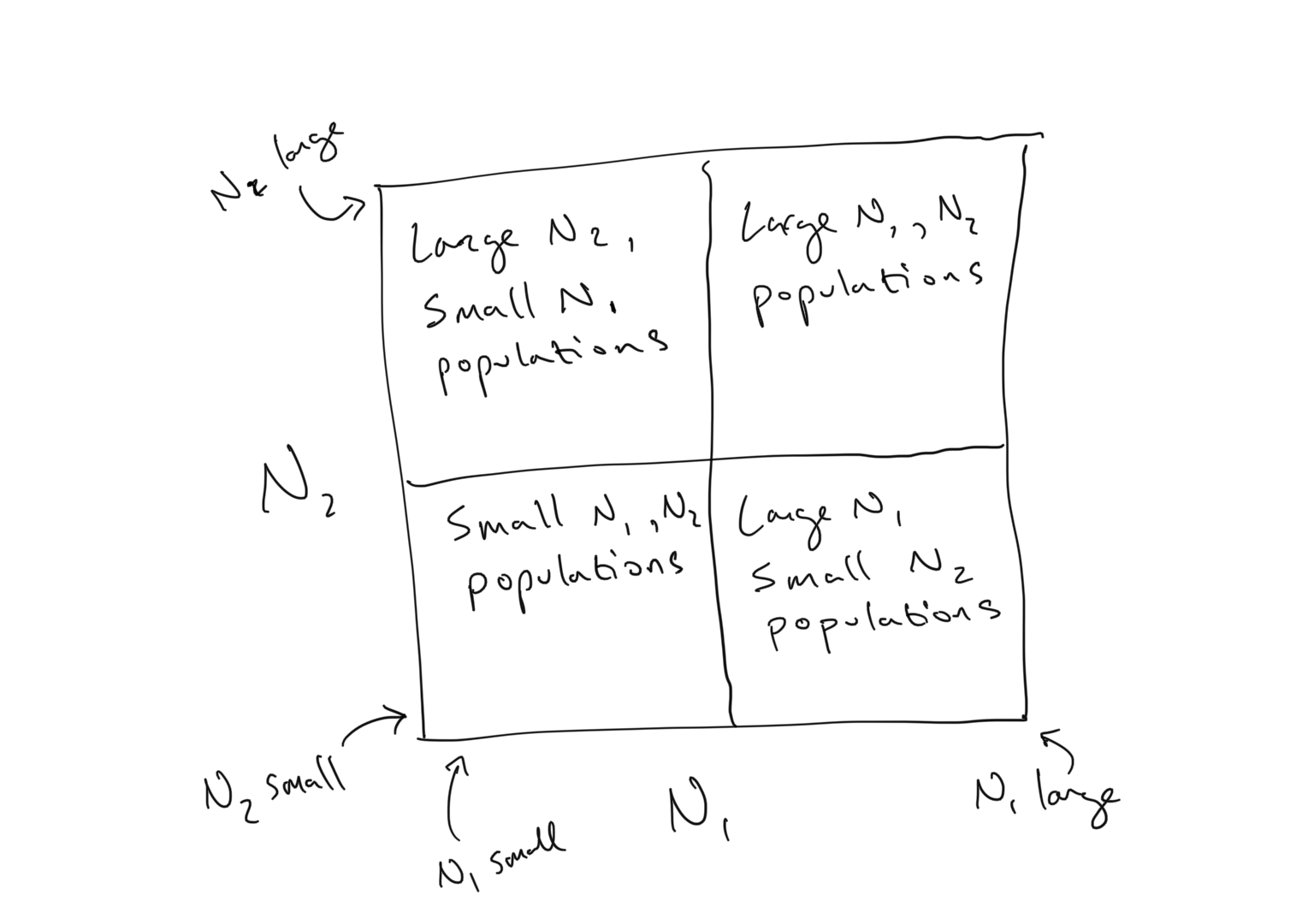
\[\begin{align} \frac{\rm d}{\rm dt}N_1 &= r_1 N_1\left( 1 - \frac{N_1 + \alpha N_2}{K_1}\right)\\ \\ \frac{\rm d}{\rm dt}N_2 &= r_2 N_2\left( 1 - \frac{N_2 + \beta N_1}{K_2}\right) \end{align}\]As we observe above, an isocline is a line along which the growth of a population is zero… i.e. a line that defines the steady state of a population. The 2-dimensional \(N_2\) vs. \(N_1\) space represented in the figures above displays any combination of population values for the species in the competition system, which we can visualize in terms of quadrants
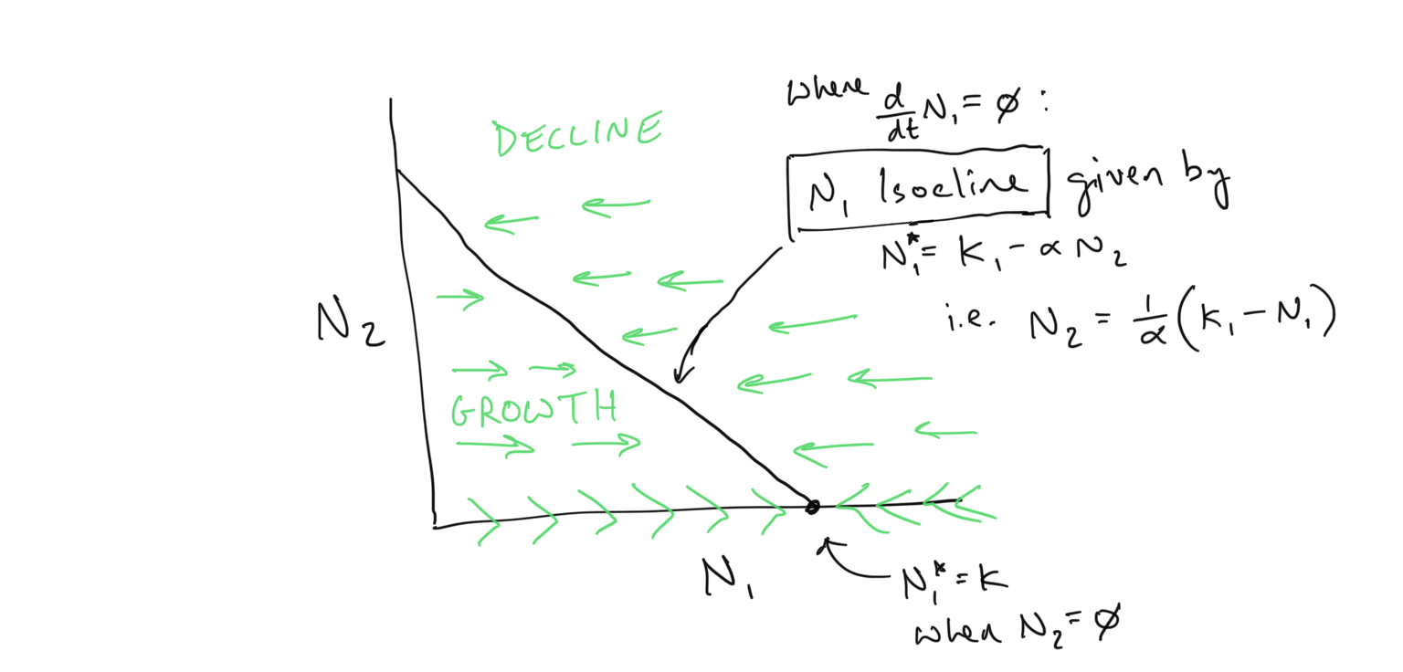
The \(N_1\) isocline within this space represents the region where \(dN_1/dt = 0\). This line is a dimensional extension of the steady state existing as a single point when we just had 1 population to consider (i.e. 1 dimension)… In 1-dimension the steady state is a point along the \(N_1\) line… in 2-dimensions the steady state is a line cutting across the \(N_2\) vs. \(N_1\) plane.
- We find the isocline by setting \(dN_1/dt = 0\)
- We reconstruct the flow by reducing the inequalities… where does the population \(N_1\) grow such that \(dN_1/dt > 0\)? Where does the population \(N_1\) decline, such that \(dN_1/dt < 0\)?
By following the algebraic steps for dealing with these inequalities as presented above, we find
- The \(N_1\) isocline is given by \(N_1^* = K_1-\alpha N_2\)
- Growth of \(N_1\) (\(\rightarrow\)) occurs when \(N_1 < K_1 - \alpha N_2\)
- Decline of \(N_1\) (\(\leftarrow\)) occurs when \(N_1 > K_1 - \alpha N_2\)
We can draw this flow within the coordinate space of \(N_2\) vs. \(N_1\) as
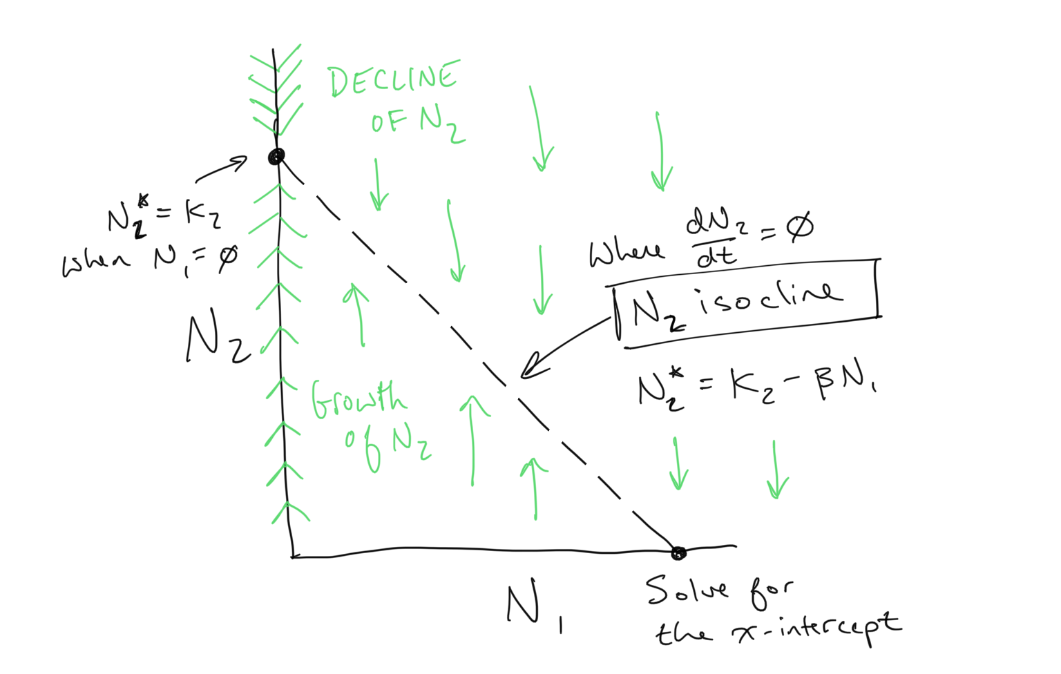
What about \(N_2\)?
You might be wondering *what about \(N_2\)? As you might guess, we now will perform the same exercise:
- Find the \(N_2\) isocline by solving for \(dN_2/dt=0\)
- Determine the flow on either side of the isocline by reducing the inequalities \(dN_2/dt < 0\) (where \(N_2\) declines) and \(dN_2/dt > 0\) (where \(N_2\) grows)
Opposite of the flow for \(N_1\), the flow of \(N_2\) as we have drawn it above will be along the vertical axis, or y-axis, because this is the axis corresponding to the population size of \(N_2\). Here is what we obtain
Discussion
- Derive the equation for the \(N_2\) isocline
- Derive the y-intercept and x-intercepts for the \(N_2\) isocline
- Compare the x,y-intercepts and slopes for the \(N_1\) and the \(N_2\) axes. What parameters determine the intercepts and slopes of each? Understanding this will be key for piecing together the dynamics of this system.
Putting it all together
We have derived the \(N_1\) isocline and we have derived the \(N_2\) isocline. We have also determined the flow along the x- and y-axes on either side of each isocline. This is all of the information we need to determine the dynamics of the Lotka-Volterra Competition model. We just need to put it together.
We will examine the dynamics for the full system by plotting both isoclines and both flow regimes in the same figure. Depending on the intercepts and slopes for the \(N_1\) and \(N_2\) isoclines, different isocline arrangements are possible, and it is these arrangements that determine the dynamics. Observe the example below
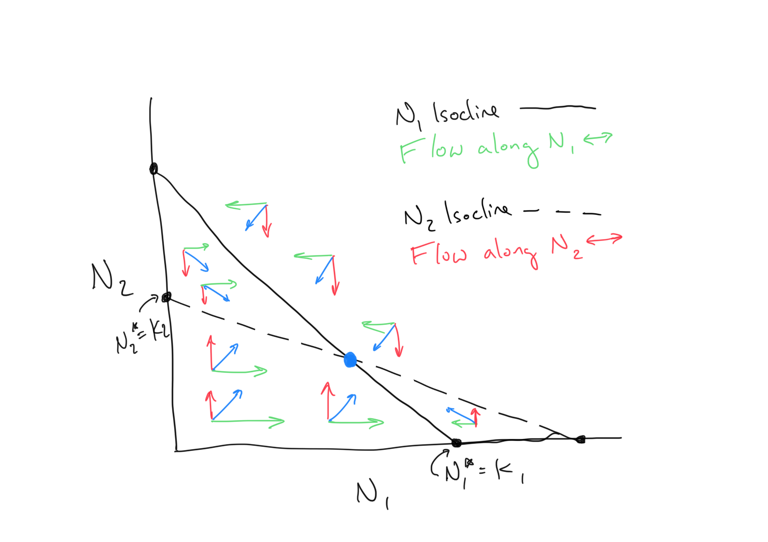
Discussion
- Judging from the figure above, what do we expect to happen to the populations of \(N_1\) and \(N_2\)?
- What does the blue point represent?
- There are three additional possible unique arrangements of the \(N_1\) and \(N_2\) isoclines depending on the relative placements of the x- and y-intercepts of both (for a total of four). Draw them and sketch out the 2-dimensional flow. What is expected to happen in each of these potential systems? How does the outcome depend on the differences in x- and y-intercepts of the \(N_1\) and \(N_2\) isoclines?
- Try solving for the point where the \(N_1\) and \(N_2\) isoclines intersect. How would you go about doing this?
Reviewing the dynamics of the LV Predator-Prey system
\[\begin{align} \frac{\rm d}{\rm dt}P &= baNP - mP \\ \\ \frac{\rm d}{\rm dt}N &= rN - aNP \end{align}\]Now that we have a better understanding of the Lotka-Volterra system and the parameters involved, let’s deploy the same tools that we used to investigate the LV competition system to understand the dynamics here. First, recall the steps required to reconstruct the dynamics of a 2-dimensional system:
- Set the \(d/dt\) equations to 0 to solve for the steady state. These will be the equations for the isoclines of the system. Here we will be finding the prey isocline (where \(dN/dt = 0\)) and the predator isocline (where \(dP/dt = 0\)).
- Find the x- and y-intercepts of the prey and predator isoclines so that we can plot them in the coordinate space where the density of prey, \(N\), is on the x-axis and the density of predators, \(P\), is on the y-axis.
- Determine the flow in the 2-dimensional space by solving for prey growth \((dN/dt > 0)\), prey decline \((dN/dt < 0)\), predator growth \((dP/dt > 0)\), and predator decline \((dP/dt < 0)\).
- From the flow along the \(N\) and \(P\) axes (i.e. flow along the horizontal and vertical axes, respectively), find the composite flow (i.e. flow along the diagonal directions).
- The composite flow will tell us how the population densities of prey \(N\) and predator \(P\) change over time, as well as the final state of the system.
First let’s examine the prey population at steady state. To derive the \(N\) Isocline, we have
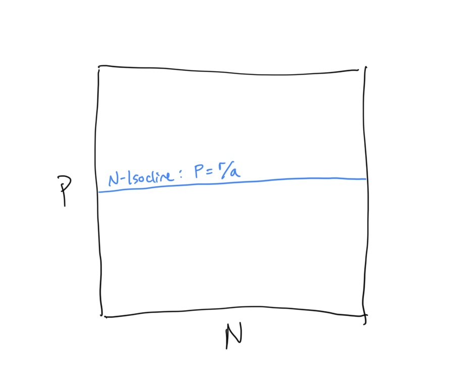
\[\begin{align} \frac{\rm d}{dt}N &= rN - aNP \\ 0 &= rN^* - aN^*P \\ rN^* &= aN^*P \\ r &= aP \\ P &= \frac{r}{a} \end{align}\]This is odd… our \(N\)-isocline is in terms of the predator population density \(P\). Keep this is mind.
Discussion
- When the prey population is at steady state \((dN/dt=0)\), the above relationship tells us where the population density of predators \(P\) falls. Given this relationship, how does a higher growth rate for prey influence the predator population density \(P\)? Provide reasoning.
- Similarly, how does a higher attack efficiency \(a\) influence predator population density \(P\)? Provide reasoning.
Let’s draw the the \(N\)-isocline in \(N-P\) space
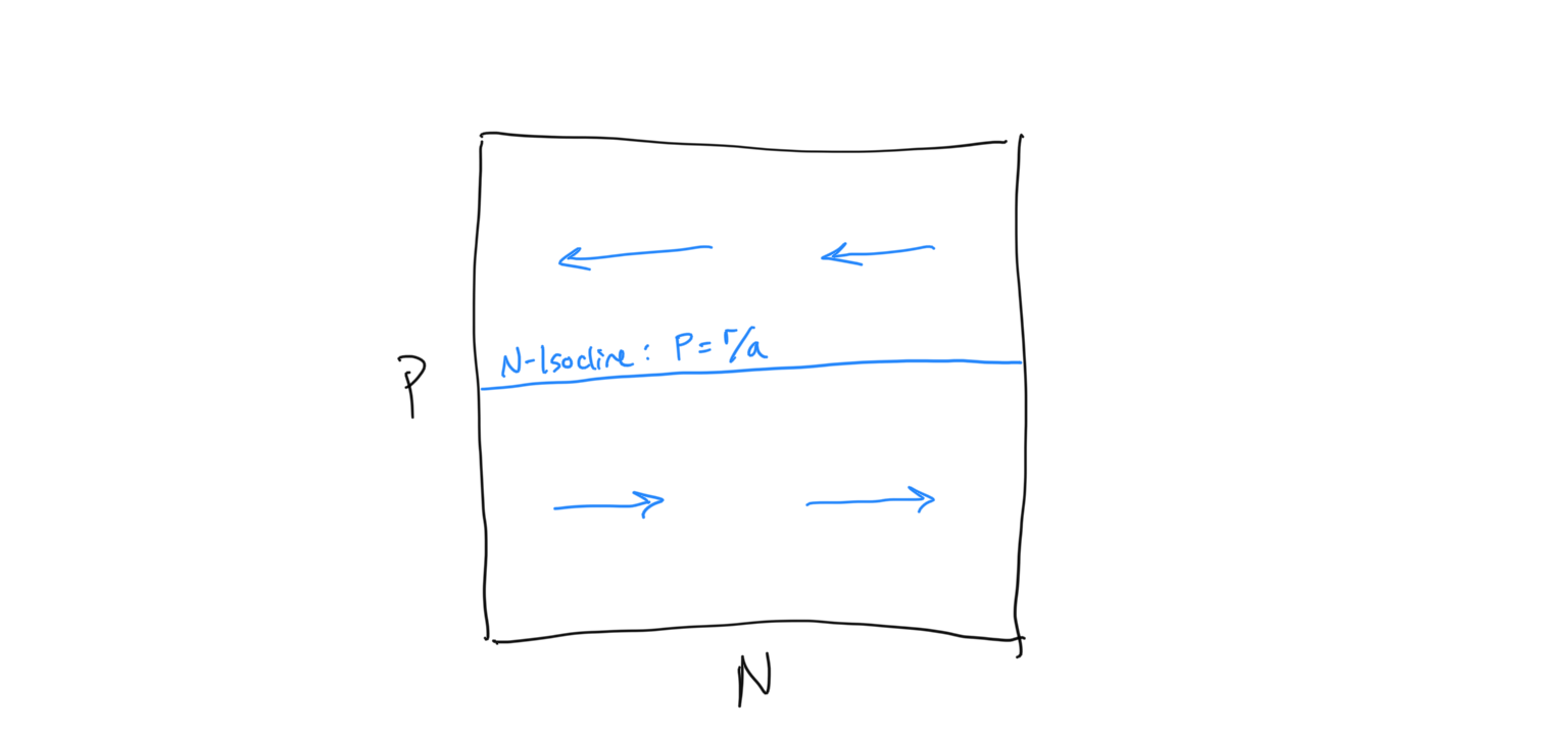
Now we need to determine the flow about the \(N\)-isocline. We do this using the same technique that we used for the competition equation. When we evaluated the competition system, we had some intuition about what was expected to happen because it built directly on the Logistic framework that we had previously investigated. Because this is a new type of system we have less intuition about how the flow should be arranged. Being very careful scientists, let’s evaluate the flow algebraically. First, let us ask when the prey population (because this is the prey isocline) is expected to increase… i.e. when is \(dN/dt > 0\)?
\[\begin{align} \frac{\rm d}{dt}N &> 0 \\ rN - aNP &> 0 \\ rN &> aNP \\ r &> aP \\ r/a &> P \\ P &< r/a \end{align}\]So when the predator density \(P\) is below the \(N\)-isocline, we have growth in the prey population \(N\). If we reverse the signs we are solving for the condition of prey population decline.\(dN/dt < 0\), which requires - unsurprisingly - that \(P > r/a\). Let us draw in the flow on either side of the \(N\)-isocline, keeping in mind that this is the flow of the prey population, which is horizontal along the x-axis.
Okay. Now let’s solve for our \(P\)-isocline, or the line along which the change in predator population over time is zero, i.e. \(dP/dt = 0\). To derive the \(P\)-isocline we have
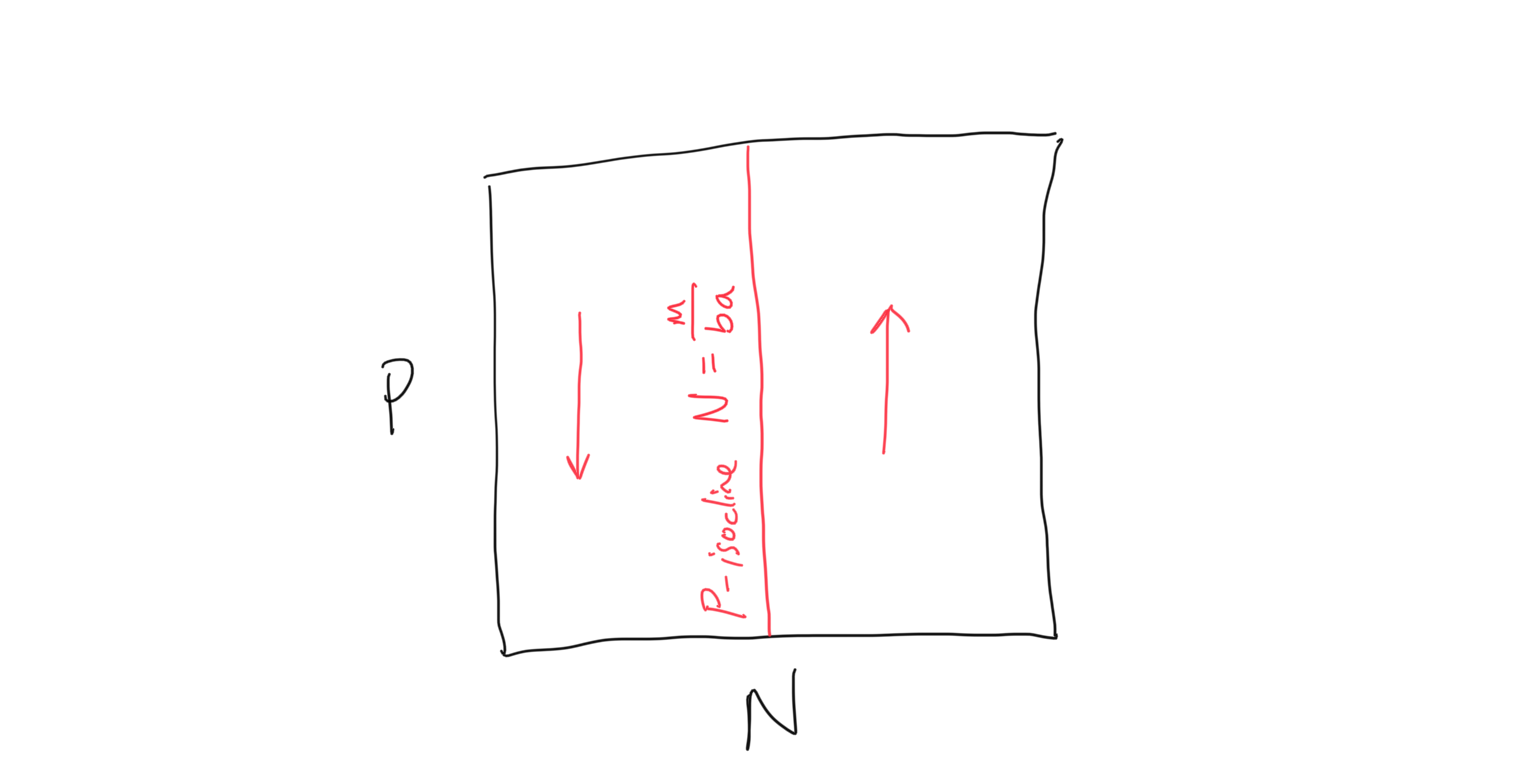
\[\begin{align} \frac{\rm d}{\rm dt}P &= baNP - mP \\ 0 &= baNP^* - mP^* \\ baNP^* &= mP^* \\ baN &= m \\ N &= \frac{m}{ba} \end{align}\]Again we have something a bit odd… this is the predator, or \(P\)-isocline, but it is in terms of the prey density \(N\)! As we will see below, this will be a vertical line in our \(P\) vs. \(N\) coordinate space. Let’s now solve for the flow on either side of this isocline. Following the same steps as before, we will ask: when will the predator population be expected to grow, so that \(dP/dt > 0\)? So
\[\begin{align} \frac{\rm d}{dt}P &> 0 \\ baNP^* - mP^* &> 0 \\ baNP^* &> mP^* \\ baN &> m \\ N &> \frac{m}{ba} \end{align}\]Because the \(P\)-isocline is \(m/ba\), this is saying that when the prey population \(N\) is greater than the \(P\)-isocline, there is growth in the predator population. And as before the inverse is true as well: when the prey population \(N\) is less than the \(P\)-isocline, there is decline in the predator population. Putting this together we see that the \(P\)-isocline and flow can be plotted
Discussion
- When the predator population is at steady state \((dP/dt=0)\), the above relationship tells us where the population density of prey \(N\) falls. Given this relationship, how does a higher mortality rate for predators influence the prey population density \(N\)? Provide reasoning.
- Similarly, how does a higher attack efficiency \(a\) and conversion efficiency \(b\) influence prey population density \(N\)? Provide reasoning.
Now let’s put the prey and predator isoclines + flow together to determine the outcome of the LV predator-prey dynamics.
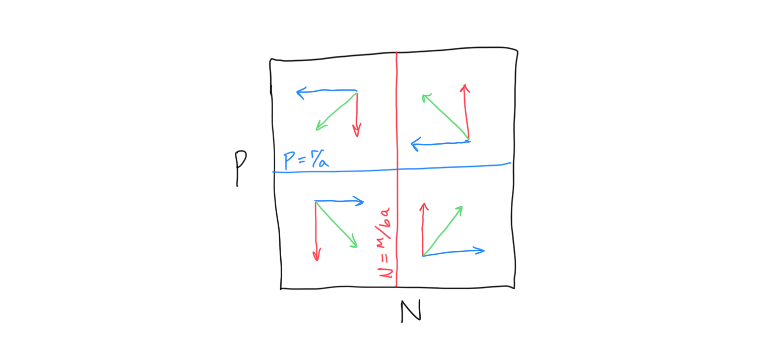
Discussion
- What are the final dynamics of the predator-prey system? On a sheet of paper, randomly pick a starting point and follow the flow. What happens?
- Translate these dynamics to a graph where you plot population sizes of the prey and predator on the y-axis against time on the x-axis. What pattern does this follow?
- Relate these expected dynamics to the Lynx-Hare system discussed in class. Are the LV predator-prey dynamics a reasonable mechanism for the observed Lynx/Hare population trajectories?
- What are the implications of these types of predator-prey dynamics with respect to the likelihood of extinction? Are populations exhibiting the dynamics expected from the LV predator-prey system ‘safe’ in terms of extinction risk? Why or why not?
- Solve for the point where \(dP/dt = 0\) and \(dN/dt = 0\). Will the system ever reach this point? If not, what is its significance?