Predator-Prey dynamics
The Lotka-Volterra Predation System
As we have investigated the dynamics of two species engaged in competitive interactions with each other, we will now use the same methodology to investigate two species engaged in a predator-prey interaction. There is one important difference here: while the Lotka-Volterra competition system is entirely symmetric (the equation for competitor \(N_1\) mirrors the equation for competitor \(N_2\)), we have to consider very different forms for the predator and prey because they interact in different (asymmetric) ways.
There are four important processes that the predator and prey equations need to capture:
- The prey species \(N\) grows exponentially in the absence of the predator
- The prey species \(N\) has a mortality caused by the predator
- The predator species \(P\) grows by consuming the prey
- The predator species \(P\) has a constant mortality rate
Let’s put these elements together into a 2-dimensional dynamic system, where we are tracking both the prey \(N\) and predator \(P\) population densities over time.
\[\begin{align} \frac{\rm d}{\rm dt}P &= baNP - mP \\ \\ \frac{\rm d}{\rm dt}N &= rN - aNP \end{align}\]Discussion
- What are the different parameters in this model, and before you read on, what do you think they mean?
- What are the units of the different parameters in this model?
- If the predator population goes extinct, what is the equation for the prey population?
- If the prey population goes extinct, what is the equation for the predator population? How does this differ from the equation for the prey population under the predator extinction condition?
What are the parameters in the LV Predator-Prey system and what do they mean?
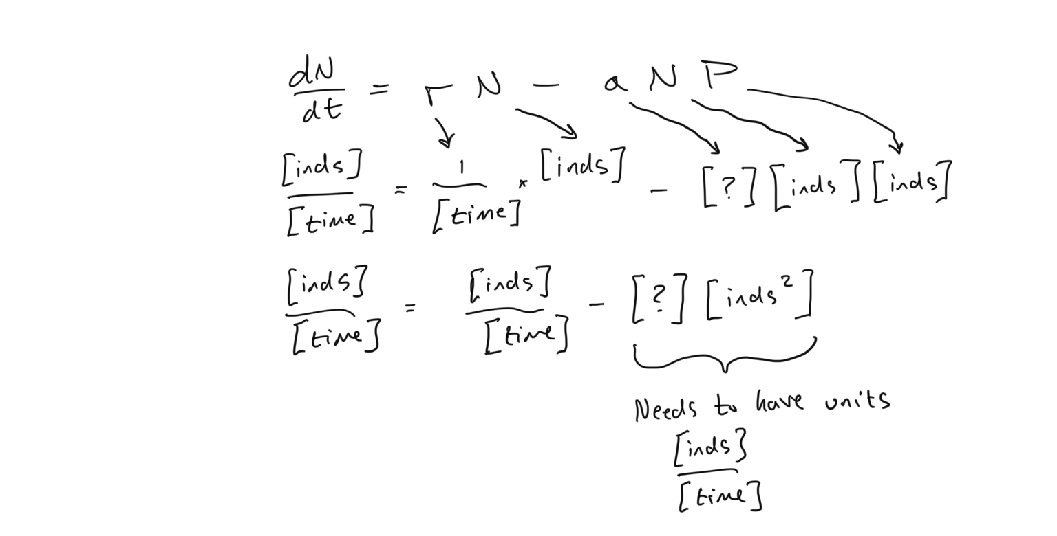
Let’s examine the different parameters that we have to consider. Let’s begin with the prey population \(N\) because one of the parameters here are already familiar to us. First, we see that the prey population \(N\) grows exponentially in the absence of a predator. The parameter \(r\), as before is the instantaneous rate of growth and has units of \(1/[time]\). The parameter \(a\) is new to us, however, and it’s units are not clear. Let’s examine the units for all of the parameters to see if we can build insight into what \(a\) represents. The central rule here is that the units of the left hand side must equal the units of the right hand side. Also it is important to remember that if we add quantities with the same unit, the result will have the same unit… in other words, if \(N\) has units of \([individuals]\) and \(P\) has units of \([individuals]\), then \(N+P\) has units of \([individuals]\). However if the terms are multiplied or divided by each other, the units take on the results of those operations. So \(N\cdot P\) has units of \([individuals^2]\)
Discussion
- What are the units of \(a\) given the unit analysis presented above? Observe that the terms \(aNP\) must have units of \([individuals]/[time]\) so that the units on the LHS (Left Hand Side) equals the units on the RHS (Right Hand Side).
- What does it mean for the change in \(N\) over time if \(a\) is large? If it is small? If it is zero? How does this aid your interpretation of its role in the LV Predator-Prey system?
As we observe in the above comparison of parameter and variable units on both sides of the equation, this new parameter \(a\) must have units of \([1/(time \times individuals)]\) for the units on both sides of the equation to match. And as you should be able to guess given the impact on \(dN/dt\) as \(a\) is increased or decreased, a larger \(a\) means that the growth of the prey is slowed down, and a smaller \(a\) means that the growth is increased. The meaning of \(a\), which will be more apparent when we examine the equation for predator growth, is the capture efficiency of prey by the predator. If a predator is more efficient (higher \(a\)), it captures more prey individuals per unit time. So the predator is more efficient at extracting prey biomass to create more predator individuals. In other words, there are more captures per prey per unit time (which corresponds to the units for \(a\) that we derived above). Now let’s examine the entire quantity \(-aNP\). From this we see that if there are more predators \(P\), there is more prey biomass taken away (and the growth of the prey declines), and that this amount scales with the population size of the prey \(N\).
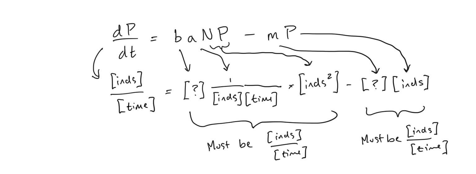
Taking what we know about \(a\), let’s examine the units of the predator equation
Discussion
- From this analysis of units, what units do the parameters \(b\) and \(m\) have?
- What is your interpretation of \(b\)?
- What is your interpretation of \(m\)?
- Do you suspect that any of the parameters in the Lotka-Volterra predator-prey system might be unitless?
- If the parameters \(r\), \(a\), \(b\) and \(m\) are higher vs. lower, how would this impact the growth of the predator population \(P\), and the prey population \(N\)? Hint: list each parameter and denote whether it has an increasing or decreasing effect on predator and prey population growth.
The parameter \(b\) is often called the conversion efficiency and varies between 0 and 1. As we can see above, whatever is taken from the prey population by the function \(-aNP\) is added to the predator population by \(+baNP\). If \(b\) varies between 0 and 1, we can see that not all biomass taken from the prey population becomes new predator biomass, and this is because much of the potential energy is lost during transfer as heat. In fact, we often assume that \(b \approx 0.1\) in most predator-prey interactions, though this number can vary substantially. It is also one of the primary reasons we are more likely to run into herbivores when out for a hike than we are to run into predators!
Discussion
- Let’s assume the ‘prey’ that we are considering is a plant species, and the ‘predator’ is an herbivore. Would \(b\) be expected to by higher or lower relative to \(b\) for a carnivore eating an herbivore? Why?
- What is the per-capita birth rate for the Predator population in terms of the parameters in the LV predator-prey system?
- What is the per-capita mortality (death) rate for the Predator population?
- What is the per-capita birth and mortality rates for the Prey population in the LV predator-prey system? (Note that for questions 2-4 the answer may be a single parameter or a combination of parameters/variables).
In summary, the Lotka-Volterra Predator-Prey system describes a prey population that grows exponentially in the absence of the predator, but that suffers mortality due to predation. On the other side, we have a predator population whose growth is tied to its consumption of the prey population… the more it consumes the higher its \(dP/dt\). The predator population cannot grow forever, as it suffers some amount of mortality proportional to its population size.
Assessing the dynamics of the LV Predator-Prey system
Now that we have a better understanding of the Lotka-Volterra system and the parameters involved, let’s deploy the same tools that we used to investigate the LV competition system to understand the dynamics here. First, recall the steps required to reconstruct the dynamics of a 2-dimensional system:
- Set the \(d/dt\) equations to 0 to solve for the steady state. These will be the equations for the isoclines of the system. Here we will be finding the prey isocline (where \(dN/dt = 0\)) and the predator isocline (where \(dP/dt = 0\)).
- Find the x- and y-intercepts of the prey and predator isoclines so that we can plot them in the coordinate space where the density of prey, \(N\), is on the x-axis and the density of predators, \(P\), is on the y-axis.
- Determine the flow in the 2-dimensional space by solving for prey growth \((dN/dt > 0)\), prey decline \((dN/dt < 0)\), predator growth \((dP/dt > 0)\), and predator decline \((dP/dt < 0)\).
- From the flow along the \(N\) and \(P\) axes (i.e. flow along the horizontal and vertical axes, respectively), find the composite flow (i.e. flow along the diagonal directions).
- The composite flow will tell us how the population densities of prey \(N\) and predator \(P\) change over time, as well as the final state of the system.
First let’s examine the prey population at steady state. To derive the \(N\) Isocline, we have
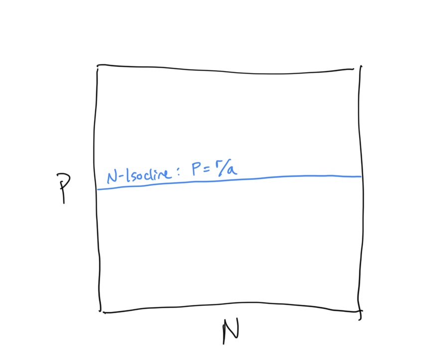
\[\begin{align} \frac{\rm d}{dt}N &= rN - aNP \\ 0 &= rN^* - aN^*P \\ rN^* &= aN^*P \\ r &= aP \\ P &= \frac{r}{a} \end{align}\]This is odd… our \(N\)-isocline is in terms of the predator population density \(P\). Keep this is mind.
Discussion
- When the prey population is at steady state \((dN/dt=0)\), the above relationship tells us where the population density of predators \(P\) falls. Given this relationship, how does a higher growth rate for prey influence the predator population density \(P\)? Provide reasoning.
- Similarly, how does a higher attack efficiency \(a\) influence predator population density \(P\)? Provide reasoning.
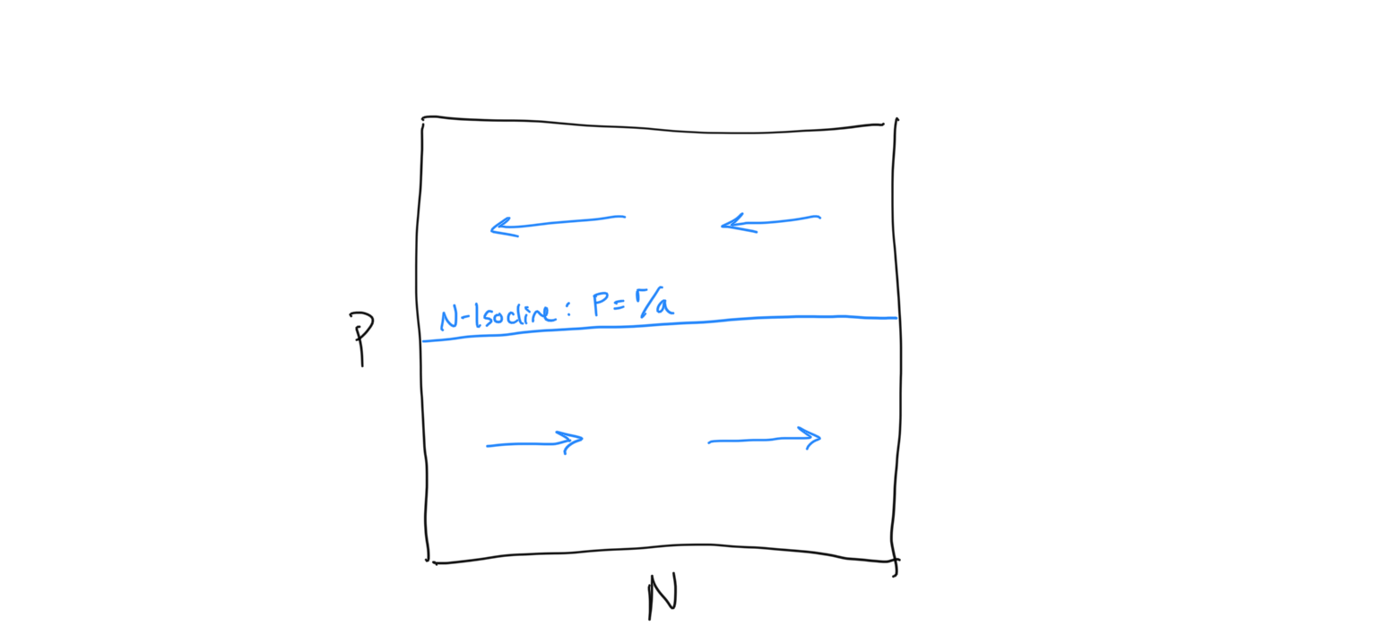
Let’s draw the the \(N\)-isocline in \(N-P\) space
Now we need to determine the flow about the \(N\)-isocline. We do this using the same technique that we used for the competition equation. When we evaluated the competition system, we had some intuition about what was expected to happen because it built directly on the Logistic framework that we had previously investigated. Because this is a new type of system we have less intuition about how the flow should be arranged. Being very careful scientists, let’s evaluate the flow algebraically. First, let us ask when the prey population (because this is the prey isocline) is expected to increase… i.e. when is \(dN/dt > 0\)?
\[\begin{align} \frac{\rm d}{dt}N &> 0 \\ rN - aNP &> 0 \\ rN &> aNP \\ r &> aP \\ r/a &> P \\ P &< r/a \end{align}\]So when the predator density \(P\) is below the \(N\)-isocline, we have growth in the prey population \(N\). If we reverse the signs we are solving for the condition of prey population decline.\(dN/dt < 0\), which requires - unsurprisingly - that \(P > r/a\). Let us draw in the flow on either side of the \(N\)-isocline, keeping in mind that this is the flow of the prey population, which is horizontal along the x-axis.
Okay. Now let’s solve for our \(P\)-isocline, or the line along which the change in predator population over time is zero, i.e. \(dP/dt = 0\). To derive the \(P\)-isocline we have
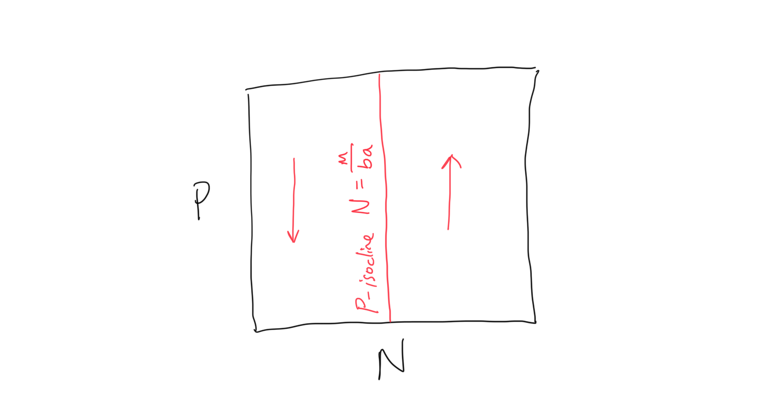
\[\begin{align} \frac{\rm d}{\rm dt}P &= baNP - mP \\ 0 &= baNP^* - mP^* \\ baNP^* &= mP^* \\ baN &= m \\ N &= \frac{m}{ba} \end{align}\]Again we have something a bit odd… this is the predator, or \(P\)-isocline, but it is in terms of the prey density \(N\)! As we will see below, this will be a vertical line in our \(P\) vs. \(N\) coordinate space. Let’s now solve for the flow on either side of this isocline. Following the same steps as before, we will ask: when will the predator population be expected to grow, so that \(dP/dt > 0\)? So
\[\begin{align} \frac{\rm d}{dt}P &> 0 \\ baNP^* - mP^* &> 0 \\ baNP^* &> mP^* \\ baN &> m \\ N &> \frac{m}{ba} \end{align}\]Because the \(P\)-isocline is \(m/ba\), this is saying that when the prey population \(N\) is greater than the \(P\)-isocline, there is growth in the predator population. And as before the inverse is true as well: when the prey population \(N\) is less than the \(P\)-isocline, there is decline in the predator population. Putting this together we see that the \(P\)-isocline and flow can be plotted
Discussion
- When the predator population is at steady state \((dP/dt=0)\), the above relationship tells us where the population density of prey \(N\) falls. Given this relationship, how does a higher mortality rate for predators influence the prey population density \(N\)? Provide reasoning.
- Similarly, how does a higher attack efficiency \(a\) and conversion efficiency \(b\) influence prey population density \(N\)? Provide reasoning.
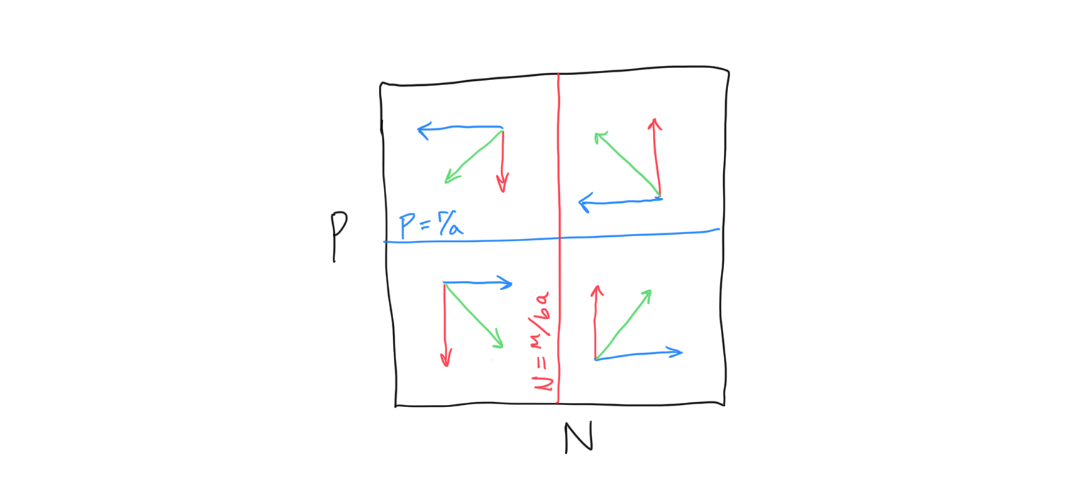
Now let’s put the prey and predator isoclines + flow together to determine the outcome of the LV predator-prey dynamics.
Discussion
- What are the final dynamics of the predator-prey system? On a sheet of paper, randomly pick a starting point and follow the flow. What happens?
- Translate these dynamics to a graph where you plot population sizes of the prey and predator on the y-axis against time on the x-axis. What pattern does this follow?
- Relate these expected dynamics to the Lynx-Hare system discussed in class. Are the LV predator-prey dynamics a reasonable mechanism for the observed Lynx/Hare population trajectories?
- What are the implications of these types of predator-prey dynamics with respect to the likelihood of extinction? Are populations exhibiting the dynamics expected from the LV predator-prey system ‘safe’ in terms of extinction risk? Why or why not?
- Solve for the point where \(dP/dt = 0\) and \(dN/dt = 0\). Will the system ever reach this point? If not, what is its significance?
Visualizing predator-prey isoclines and dynamics
Below is a code block where the Lotka Volterra predatpr-prey system is simulated. The main plot will show the predator \(P\) (red) and prey \(N\) (blue) isoclines, as well as the starting point and trajectory of the \(P\) and \(N\) populations over time (green circle and line, respectively). On the top right inset is a plot of the two \(P\) and \(N\) population sizes plotted over time. Make sure that you understand how the isoclines determine the flow and direct how the combined trajectories of \(P\) and \(N\) (green) change over time, and how this corresponds to the population sizes shown in the inset.
Try changing the values of the parameters. Based on your derived equations for the \(P\) and \(N\) isoclines, try to anticipate what the changes you make will do to the predator/prey dynamics.
    library(RColorBrewer)
    library(deSolve)
    pal = brewer.pal(3,'Set1')
    # Define the Rates function
    pred.flow = function(r,a,b,m,Pstart,Nstart,tmax) {
        # LV.comp = function(r1,r2,alpha,beta,K1,K2,N1start,N2start,tmax) {
        yini = c(P = Pstart,N = Nstart)

        fmap = function (t, y, parms) {
        with(as.list(y), {
            dP <- b*a*y[2]*y[1] - m*y[1]
            dN <- r*y[2] - a*y[2]*y[1]
            list(c(dP,dN))
        })
        }

        times <- seq(from = 0, to = tmax, by = 0.1)
        out   <- ode(y = yini, times = times, func = fmap, parms = NULL)

        Ptraj = out[,2];
        Ntraj = out[,3];
        timeline = out[,1];

        Pend = tail(Ptraj,n=1)
        Nend = tail(Ntraj,n=1)

        maxtraj = max(c(Ptraj,Ntraj));

        Psize = maxtraj*1.2;
        Nsize = maxtraj*1.2;

        p_isocline = m/(b*a); # = N
        n_isocline = r/a; # = P

        par(fig = c(0,1,0,1))
        plot(rep(p_isocline,100),seq(-10,Psize,length.out=100),type='l',lwd=2,col=pal[1],xlim=c(0,maxtraj*1.2),ylim = c(0,maxtraj*1.2),xlab='N population',ylab='P population',lty=2)
        lines(seq(-10,Nsize,length.out=100),rep(n_isocline,100),lwd=2,col=pal[2],lty=2)
        points(Nstart,Pstart,pch=16,cex=2,col=pal[3])
        lines(Ntraj,Ptraj,col=pal[3],lwd=2)
        points(Nend,Pend,pch=8,cex=2,col=pal[3])
        legend(0,maxtraj*1.2,c('P isocline','N isocline'),pch=16,col=pal)

        par(fig = c(0.5,1, 0.5, 1), new = T)
        plot(timeline,Ptraj,type='l',col=pal[1],xlab='Time',ylab='Pop. size',lwd=2,ylim = c(0,maxtraj))
        lines(timeline,Ntraj,type='l',col=pal[2],lwd=2,)

    }
    # Plug in parameter values and run
    pred.flow(r = 0.5, a = 0.01, b = 0.1, m = 0.1, Pstart = 70, Nstart = 100, tmax = 500)