< Back to Course Page

This is an except from a Discussion Section for Foundations of Ecology, but it is useful, I think for getting re-acquainted with some basic population dynamics…

Examine Logistic Population growth, where \(r\) is the instantaneous rate of growth, \(K\) is the carrying capacity, \(tmax\) is the maximum number of timesteps, and \(N0\) is the initial population size.

    library(deSolve)
    pop.logistic2 = function(r,K,tmax,N0) {
        yini = c(N = N0)
        
        fmap = function (t, y, parms) {
        with(as.list(y), {
            dN <- r*N*(1 - (N/K))
            list(dN)
        })
        }
        
        times <- seq(from = 0, to = tmax, by = 0.1) 
        out   <- ode(y = yini, times = times, func = fmap, parms = NULL)
        
        plot(out, lwd = 2,xlab='Time',ylab='Population N(t)')
    }
    pop.logistic2(r = 0.01,K = 30,tmax = 1000,N0 = 1)

Discussion

1. Try alternative values for r and K. How do these parameters impact the dynamics of the population when you start at different population sizes N0?

Flow Diagram for the Logistic Equation

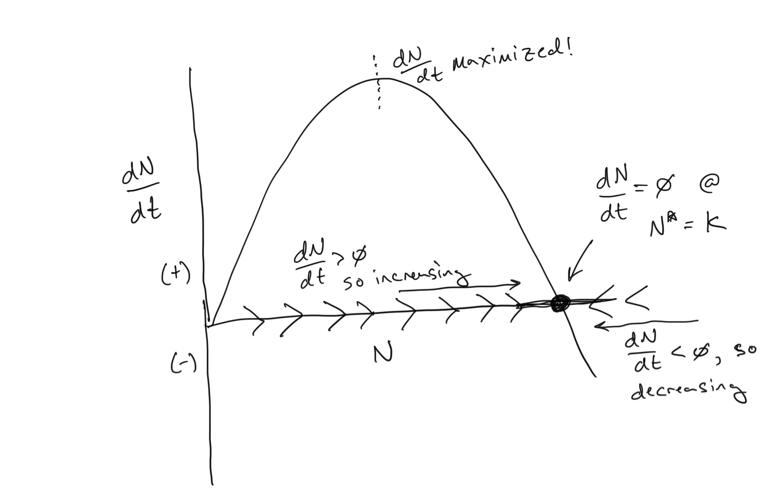
Our population growth equation that incorporates density-dependent per-capita birth and death rates is known as the Logistic Equation. You can see above how it has a sigmoidal shape… population growth begins exponentially but then tapers off as it reaches the carrying capacity \(K\). And we have used the per-capita birth and death rates to anticipate the dynamics using the flow concept. Below we see that we can use the flow concept in a different way… to examine \(dN/dt\) as a function of \(N\).

Discussion

1. Where is the carrying capacity \(K\)?
2. There are two values of \(N\) where \(dN/dt = 0\). What are they?
3. Where is \(dN/dt\) maximized on the plot above? Can you guess the value of \(N\) corresponding to where \(dN/dt\) is maximized? What is special about this point in terms of how the population changes over time?
4. Bonus round: Can you analyitically solve for the point at where \(dN/dt\) is maximized in terms of \(N\)? Hint: to do this you would need to take the derivative of something…

Part II: Discrete Population Growth

Continuous Back to Discrete!

Now let’s decouple the time-step size in the first equation with the goal of turning it into a discrete process. First, we should define \({\rm d}/{\rm dt}\)…

where the \(\lim\) notation means that we are evaluating the function at the limit of \(\Delta t \rightarrow 0\) (this is a foundational concept in Calculus… it means we are assuming the size of the time step is really really really small), and where we specify that the growth rate here is with respect to a (now) discrete-time system via the subscript \({}_d\). Now let’s imagine that \(\Delta t\) is not really really really small such that the \(\lim_{\Delta t \rightarrow 0}\) can be ignored… in fact, let’s assume that \(\Delta t\) is quite large. Because it is large, it’s significance is important, and we will multiply it to both sides of the equation to obtain

To obtain an equation for \(N(t)\) for a discrete time system, we use recursion, which we discussed in class. Following the procedure outlined in lecture we obtain

where \(\lambda = N(t+1)/N(t)\).

Discussion

1. Relate \(\lambda\) to the instantaneous rate of growth \(r\). In other words, solve for \(\lambda\) in terms of \(r\), and solve for \(r\) in terms of \(\lambda\). *Hint: do this by utilizing both continuous- and discrete-time definitions for \(N(t)\).
2. What does \(\lambda\) represent compared to \(r\), and how do different values of each correspond to increasing, decreasing, and steady state population dynamics? Plug in some values for each and experiment.
3. If \(r = 0.02~{\rm year}^{-1}\), what is \(\lambda\) in a corresponding discrete-time system?
4. What are \(r\) and \(\lambda\) at steady state? I.e. at the condition where the change in population size is zero over time?
5. We discussed in class how to calculate the doubling time for a population according to continuous-time dynamics. Using the discrete time solution for \(N(t)\), what is the equation for doubling time for a discrete-time population? How does this compare to the doubling time of a continuous-time population? Hint: Solve \(2N_0 = N_0 \lambda^t\) for \(t\).

Discrete logistic population growth

We have spent a significant amount of time in class deriving the Logistic Population equation for continuous-time dynamics. Now let’s explore a discrete-time version of the logistic equation. For your reference, both the continuous-time (top) and discrete-time (bottom) versions of the logistic equation are presented below.

Think carefully about the differences, and remember that \(N(t+1) - N(t) = \Delta N\), or ‘the change in \(N\). Also note that here \(\Delta t = 1\). Let’s consider whether our expectations for the discrete logistic should be the same or different than the continuous logistic.

Discussion

1. What should \(\Delta N\) approximate if \(N \approx 0\)? Compare this to the same expectation for the continuous-time \({\rm d}N/{\rm dt}\).
2. Do the same for \(N \approx K\).

Okay… so let’s now see if our expectations match reality. Below is a code block where the discrete logistic is simulated over time. As with the continuous-time population equation, we have to supply the initial population size \(N_0\), and the (in this case) discrete growth parameter \(r_d\) and the carrying capacity \(K\). In addition we have to specify the number of time-steps over which we will simulate tmax.

For simplicity, let’s keep K=1 for now. Recall that in class, \(N^* = K\), which means that the steady state for the continuous-time system is at the carrying capacity \(K\). But if \(K=1\), what does this mean? The steady state is at 1 individual??? No - this wouldn’t make sense. Remember that \(N\) could be in units of \([individuals]\) (where only integer values make sense) or could be in units of density \([individuals/area]\). In the case of the latter, fractional values have meaning… for example, let’s consider 0.1 individuals/area. If our area is in units of \([{\rm km}^2]\), 0.1 \(individuals/km^2\) means that there is roughly 1 individual per 10 \({\rm km}^2\). If \(K=1\), then we can assume that we are dealing with densities.

Run the code block below, and see if your expectations for \(N \approx 0\) and for \(N \approx K\) are correct, where in this case \(K=1\).

    logistic.map = function(rd,K,N0,tmax) {
        N = numeric(tmax)
        N[1] = N0
        for (t in 2:tmax) {
            Nt = N[t-1] + rd*N[t-1]*(1 - N[t-1]/K)
            N[t] = Nt 
        }
        plot(N,type='l')
    }

    logistic.map(rd = 1, K = 1,N0=0.01,tmax=30)

Discussion

1. Now set rd = 2. What dynamics do you observe? Describe them. Are they stable?
2. Set rd = 2.5. What dynamics do you observe? Describe them. Are they stable?
3. Set rd = 3.0. What dynamics do you observe? Describe them. Are they stable? Not clear? Change tmax = 100 to give you a longer-time perspective. How would you describe what you see?

Cobweb Diagrams

For the continuous-time logistic equation, we were able to learn a lot about the dynamics of the system by graphically analyzing the ‘flow’ when we plotted \({\rm d}N/{\rm dt}\) (on the y-axis) versus \(N\) (on the x-axis). There is an analogous method for the discrete time logistic equation, however there is a little more to it that requires careful consideration.

For the discrete-time system, we will graphically analyze the plot of \(N(t+1)\) (on the y-axis) as a function of \(N(t)\) (on the x-axis). As with the continuous-time equation, this produces a parabola. The parabola represents the mapping from \(N(t)\) to \(N(t+1)\). In other words, if our population is at value \(N(t)\), to find the next value at time \(t+1\), we identify the value of \(N(t)\) on the x-axis, draw a vertical line up to the parabola, and this gives us the value at \(N(t+1)\). We then reiterate the process. We can make life simpler for ourselves if we also draw the 1:1 line in the same plot (where \(N(t) = N(t+1)\)). Instead of going back to the x-axis for every \(N(t)\) to draw the vertical line up to the parabola (giving us \(N(t+1)\)), we can simply draw a horizontal line to the 1:1 line (resetting \(N(t+1)\) to \(N(t)\)), and than a vertical line up or down to the parabola to get at the next value of \(N(t+1)\). Below we observe the process for tracing the dynamics of a discrete time system in this way:

• First, find \(N(t)\) on the x-axis
• Draw a vertical line up to the parabola. This is \(N(t+1)\)
• Draw a horizontal line over to the 1:1 line. This resets \(N(t)\) along the x-axis
• Draw a vertical line up or down to the parabola. This gives us \(N(t+1)\)
• Draw a horizontal line over to the 1:1 axis
• Repeat, repeat, repeat!

The above algorithm constitutes what we call a cobweb diagram. We implement this algorithm via simulation in the code block below. Run the same parameter sets that you encoded above into the cobweb diagram below. Make sure you understand what the cobweb diagram is showing. Confirm that the time-simulation of the discrete-logistic equation and the cobweb diagram are telling us the same thing.

    logistic.cobweb = function(rd,K,N0,tmax) {
        N = numeric(tmax)
        N[1] = N0
        for (t in 2:tmax) {
            Nt = N[t-1] + rd*N[t-1]*(1 - N[t-1]/K)
            N[t] = Nt 
        }
        Ntx = seq(0,max(N)*(1+0.5),length.out=100)
        Nty = Ntx + rd*Ntx*(1 - Ntx/K)
        xymax = max(N)
        plot(Ntx,Nty,type='l',xlab="Population size N(t)", ylab="Population size N(t+1)",lwd=2,xlim=c(0,xymax),ylim=c(0,xymax))
        lines(seq(-1,2),seq(-1,2),col='gray',lwd=2)
        for (t in 1:(tmax-1)) {
            #draw segments
            segments(x0=N[t],y0=N[t],x1=N[t],y1=N[t+1],col='blue')
            segments(x0=N[t],y0=N[t+1],x1=N[t+1],y1=N[t+1],col='blue')
        }
    }
    logistic.cobweb(rd = 1, K = 1, N0=0.01, tmax=40)

Discussion

1. Across intervals of 0.1, at what value of \(r_d\) do the dynamics become cyclic? Unpredictable?
2. Compare rd=1.8 to rd=2.0. What is the primary difference between these outcomes. Compare both the results of the cobweb diagram and the \(N(t)\) vs. \(t\) plot to establish your interpretation of what is going on.
3. Do we observe cycles or chaotic dynamics in the continuous-time logistic model? (Below is the code block from Section 7 where we assessed continuous-time logistic dynamics, which you can use for reference)
4. Given these differences, what are the long-term implications for discrete-time vs. continuous-time population dynamics?
5. What ecological factors might promote continuous- vs. discrete-time population dynamics?

Compare the Continuous- and Discrete-time systems directly

This code block allows us to directly compare the temporal dynamics of continuous-time and discrete-time logistic populations directly. Use this to inform your answers to the above questions.

    library(deSolve)
    pop.combined = function(r,K,N0,tmax) {
        #Continuous model
        yini = c(N = N0)
        fmap = function (t, y, parms) {
        with(as.list(y), {
            dN <- r*N*(1 - (N/K))
            list(dN)
        })
        }
        
        times <- seq(from = 1, to = tmax, by = 0.1) 
        out   <- ode(y = yini, times = times, func = fmap, parms = NULL)
        
        # Discrete model
        Nd = numeric(tmax)
        Nd[1] = N0
        for (t in 2:tmax) {
            Ndt = Nd[t-1] + r*Nd[t-1]*(1 - Nd[t-1]/K)
            Nd[t] = Ndt 
        }
        maxN = max(c(Nd,out[,2]))
        plot(out, lwd = 2,xlab='Time',ylab='Population N(t)',col='blue',ylim=c(0,maxN))
        lines(Nd,col='red',lwd=2)
    }
    pop.combined(r = 1,K = 1,N0 = 0.01,tmax = 40)