Section 9 :: Carrying Capacity to Competition
Carrying Capacity
We have shown how discrete-time population growth relates to continuous-time population growth. We are now going to stick with continuous time population dynamics (we will spend an entire section next week back in discrete time).
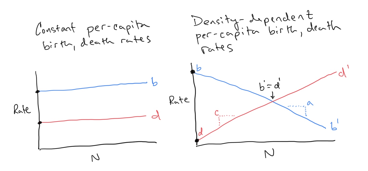
Exponential population growth occurs when the environment and resources are not limiting, and is usually observed at the beginning of a species’ colonization/invasion of a new habitat. However, as the population grows individuals consume resources and space. Eventually this feeds back to influence the rate at which the population is growing. In terms of our equation for population growth, we can say that the per-capita birth and death rates might be expected to change as the environment fills up with individuals. So where before we said total births \(B\) and deaths \(D\) were density-dependent (linear function of \(N\) with slopes given by constant per-capita birth and death rates \(b\) and \(d\)), now we are saying that these per-capita birth and death rates should not be constant, but also change with population size \(N\).
Discussion
- These population equations generally only track females within sexually-reproducing populations. Why?
- Why did we choose birth rates to decrease with increasing \(N\) and death rates to increase with increasing \(N\)?
- For the figures shown on the left and right, we have drawn how per-capita birth and death rates change (or not) as a function of population size. Similar to how we related the fitness of a morph to changes in its proportion within a population, we can reconstruct the flow of the population along the x-axis by observing the relationship between per-capita birth and death rates. When should flow increase and when should flow decrease? Remember that the x-axis is population size \(N\). We are asking when should the population increase and when should it decrease given some combination of per-capita birth and death rates. On the figures above can you use the concept of flow to predict what will happen to the populations?
- What if we swapped the definitions for birth and death rates? Can you use the concept of flow to anticipate what will happen to the population?
As we will (or have?) explore(d) in class, we can write down equations for density-dependent per-capita birth and death rates as
\[\begin{align} b^\prime &= b - aN \\ d^\prime &= d + cN \end{align}\]This explicitly encodes the idea that births decease with increasing \(N\) and deaths increase with increasing \(N\). Note also that the y-intercept for the per-capita birth rate is \(b\) and that the y-intercept for the per-capita death rate is \(d\). In other words, when \(N\) is close to zero (i.e. the population is very very small), the per-capita birth rate \(b^\prime \approx b\) and the per-capita death rate \(d^\prime \approx d\) (where \(\approx\) means is approximately or is close to). As we have defined \(r = b - d\), we can define a density dependent \(r^\prime = b^\prime - d^\prime\).
Let’s substitute this into the continuous-time equation for population growth:
\[\begin{align} \frac{\rm d}{\rm dt}N &= r^\prime N \\ \\ \frac{\rm d}{\rm dt}N &= (b^\prime - d^\prime)N \\ \\ \frac{\rm d}{\rm dt}N &= \left( (b - aN) - (d + cN) \right)N \\ \\ \frac{\rm d}{\rm dt}N &= (b-d)N\left( 1 - \frac{(a+c)}{(b-d)}N \right) \\ \\ \frac{\rm d}{\rm dt}N &= rN\left( 1 - \frac{(a+c)}{(b-d)}N \right) \end{align}\]…and to remind us of the meaning of these parameters:
- \(r\) = intrinsic rate of growth (now specifically when the population is small)
- \(b\) = per-capita birth rate when the population is small
- \(d\) = per-capita death rate when the population is small
- \(a\) = the slope at which births decline with increasing population size
- \(c\) = the slope at which deaths incline with increasing population size
Discussion
- Use algebraic manipulation to derive the 4th equation in the list above from the 3rd equation
We can simplify this a little bit. Let’s define a new parameter
\[\begin{align} K &= \frac{b-d}{a+c},~{\rm or} \\ \\ \frac{1}{K} &= \frac{a+c}{b-d} \end{align}\]Substituting this term in above gives us
\[\begin{equation} \frac{\rm d}{\rm dt}N = rN\left(1 - \frac{N}{K} \right) \end{equation}\]Now let’s investigate how changes in \((r,b,d,a,c)\) impact the dynamics of the system in exactly the same way that we did before with respect to individual fitness. However, instead of visualizing which phenotypic fitness measure was greater or less than the other, we will examine when per capita birth rates are greater than death rates (population growth) and when per capita death rates are greater than birth rates (population decline).
    # Define the Rates function
    pop.flow = function(b,d,a,c) {

        # Population size
        N = seq(0,100,5)

        # Define per-capita birth and death rates
        pcbr = b - a*N
        pcdr = d + c*N

        # Plot percapita birth and death rates as a function of N
        plot(N,pcbr,type='l',col='blue',lwd=2,ylim=c(min(c(pcbr,pcdr)),max(c(pcbr,pcdr))),xlab='Population Size (N)',ylab='Rate')
        lines(N,pcdr,col='red',lwd=2)
        legend(0.8,max(c(pcbr,pcdr)),c('p-c birth rate','p-c death rate'),pch=15,col=c('blue','red'))

        # Add flow information
        text(1,(1-0.25)*min(c(pcbr,pcdr)),'Flow',cex=1.5)
        for (i in 1:length(N)) {
            loc = i
            if (pcbr[loc] > pcdr[loc]) {
                text(N[i],min(c(pcbr,pcdr)),'>',cex=1.5)
            }
            if (pcbr[loc] < pcdr[loc]) {
                text(N[i],min(c(pcbr,pcdr)),'<',cex=1.5)
            }
            if (pcbr[loc] == pcdr[loc]) {
                text(N[i],min(c(pcbr,pcdr)),'--',cex=1.5)
            }
        }
    }
    # Plug in parameter values and run
    pop.flow(b = 0.8, d = 0.2, a = 0.01,c = 0.01)
Discussion
- Given
r = 0.01,b = 0.8, d = 0.2, a = 0.01,c = 0.01, where does the flow indicate that the population will settle?- Plug in the values \((b,d,a,c)\) to solve for \(K\) given the equation for \(K\) above. Comparing this value to what we observe in the graph, what is our interpretation of what \(K\) means?
- Let’s a) switch
banddand reverse the direction of the slope, so that our parameters arer = 0.01,b = 0.2, d = 0.8, a = -0.01,c = -0.01. How do we interpret what will happen to this population? Is this realistic?- Derive the y-intercepts and x-intercepts for \(b^\prime\) and \(d^\prime\) in terms of \((b,d,a,c)\). Can you confirm analytically the x- and y-intercepts that you observe in the above graph?
We are now going to use a differential equation solver to examine how \(N(t)\) changes over time \(t\). This is a numerical method for observing the dynamics of a differential equation system without having to solve for \(N(t)\). In fact, we can solve for \(N(t)\) using integration by parts (shudder), but we won’t go there in this class.
    library(deSolve)
    # Define the logistic growth dynamic model
    pop.logistic = function(b,d,a,c,tmax,N0) {
        yini = c(N = N0)

        fmap = function (t, y, parms) {
        with(as.list(y), {
            dN <- (b-d)*N*(1 - ((a+c)/(b-d))*N)
            list(dN)
        })
        }

        times <- seq(from = 0, to = tmax, by = 0.1)
        out   <- ode(y = yini, times = times, func = fmap, parms = NULL)

        plot(out, lwd = 2,xlab='Time',ylab='Population N(t)')
    }
    # Plug in parameter values and run
    pop.logistic(b = 0.8, d = 0.2, a = 0.01,c = 0.01,tmax = 1000,N0 = 1)
Discussion
- Input the initial parameter combinations that we investigated in the flow diagram. How does this plot compliment our expectations of the dynamics from predicting the flow?
- Unlike the flow diagram, we have to input an initial population size \(N_0\). Try entering a large \(N_0\) as the starting population. What do you observe? Does the long-term dynamics change?
- What is the role in
r? How does changingrchange what happens to the population?- As before, let’s a) switch
banddand reverse the direction of the slope, so that our parameters arer = 0.01,b = 0.2, d = 0.8, a = -0.01,c = -0.01, tmax = 1000,N0 = 1. Try this for \(N_0 = 1\), \(N_0 = 29\), \(N_0 = 30\), and \(N_0 = 31\). Does what you observe match your expectations for what you predicted the population to do from the flow diagram? Why do you think you got an error message for \(N_0 = 31\)?
Finally, let’s check out a simplified version of what we have above. Instead of changing \((b,d,a,c)\), we will used the compressed notation, where we assess population dynamics in terms of \((r,K)\).
    library(deSolve)
    pop.logistic2 = function(r,K,tmax,N0) {
        yini = c(N = N0)

        fmap = function (t, y, parms) {
        with(as.list(y), {
            dN <- r*N*(1 - (N/K))
            list(dN)
        })
        }

        times <- seq(from = 0, to = tmax, by = 0.1)
        out   <- ode(y = yini, times = times, func = fmap, parms = NULL)

        plot(out, lwd = 2,xlab='Time',ylab='Population N(t)')
    }
    pop.logistic2(r = 0.01,K = 30,tmax = 1000,N0 = 1)
Discussion
- Try alternative values for
randK. How do these parameters impact the dynamics of the population when you start at different population sizesN0?
Flow Diagram for the Logistic Equation
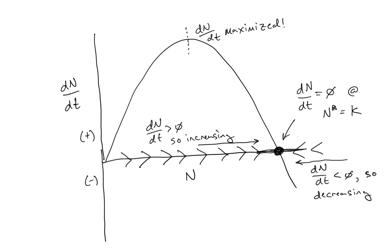
Our population growth equation that incorporates density-dependent per-capita birth and death rates is known as the Logistic Equation. You can see above how it has a sigmoidal shape… population growth begins exponentially but then tapers off as it reaches the carrying capacity \(K\). And we have used the per-capita birth and death rates to anticipate the dynamics using the flow concept. Below we see that we can use the flow concept in a different way… to examine \(dN/dt\) as a function of \(N\).
Discussion
- Where is the carrying capacity \(K\)?
- There are two values of \(N\) where \(dN/dt = 0\). What are they?
- Where is \(dN/dt\) maximized on the plot above? Can you guess the value of \(N\) corresponding to where \(dN/dt\) is maximized? What is special about this point in terms of how the population changes over time?
- Bonus round: Can you analyitically solve for the point at where \(dN/dt\) is maximized in terms of \(N\)? Hint: to do this you would need to take the derivative of something…
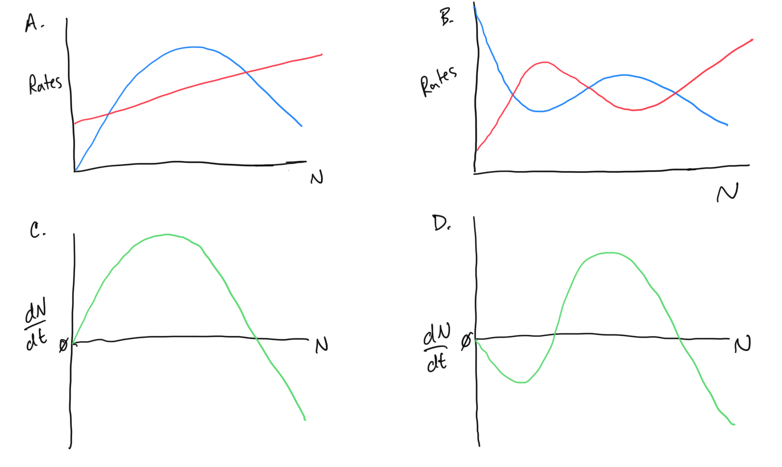
Interpret the following diagrams
Make sure that you understand what all of the relationships mean and can elucidate expectations for what the population will do over time! I recommend that you either a) print out the below figure, or better yet b) transcribe it yourself onto a sheet of paper so that you can draw and label the various elements to help you interpret what is going on.
Discussion
- For each of the above diagrams… where are the steady states? What is the flow above or below the steady states? What will happen to the population given that it starts at various places along the x-axis?
- In which diagrams can you say something about how quickly the population changes over time? Where is population change fast, where is it slow?
- In which diagrams is there an Allee effect (if any)? Why?
Including the basics effects of competition!
We will now consider a second species, with population density \(C\). For now, we will not assume that \(C\) changes over time… so it is a constant. The population of the competitor \(C\) will stay the same even as \(N\) changes over time (we will relax this assumption in the next section). The population of \(C\) has a negative effect on the population of \(N\), very similar to how a larger population \(N\) is expected to limit resources, slowing down \({\rm d}N/{\rm dt}\) as codified in the Logistic Equation.
Let’s state some assumptions… if individuals in population \(C\) are doing the same things (for example using the same resources) as individuals in population \(N\), we expect them to have the same effect on slowing down the growth of population \(N\). If the individuals in population \(C\) are doing very different things (for example using mostly different resources) as individuals in population \(N\), we expect them to have less of an effect on the growth of population \(N\).
Let’s introduce a parameter \(\alpha\) that captures this relationship. If \(\alpha=1\) we will say that the competitors \(C\) are using the same resources as the population \(N\). If \(\alpha < 1\), we will say that the competitors are using very different resources. So now let’s introduce this into the Logistic Equation:
\[\begin{equation} \frac{\rm d}{\rm dt}N = rN\left( 1 - \frac{N + \alpha C}{K}\right) \end{equation}\]Discussion
- Explore this equation. What does it mean if \(\alpha = 1\) or if \(\alpha < 1\) (assume that \(\alpha\) remains strictly positive). What does it mean if the size of the competitors population \(C\) is large or small for a given value of \(\alpha\)? In other words, how do these variations impact \({\rm d}N/{\rm dt}\)?
- Solve for \({\rm d}N/{\rm dt} = 0\). How does introducing a competitor alter our expectations from Logistic Growth?