Section 5 :: Life History Strategies

< Back to Course Page

As we are learning in class, species display a wide variety of life histories. From a relatively simple perspective, a species’ life history accounts for the scheduling, timing, duration, and effort of various behaviors that impact its accumulated fitness at the end of an individual’s life, or lifetime fitness, which we will represent by the symbol \(\Phi\). Let’s consider a few examples where fitness is evaluated by accounting for the energetic investment in offspring.

• Mosquitos give birth to an enormous number of offspring, but invest very little energy into each one. As such, the probability that an individual mosquito larvae dies is high, but there are still a lot of mosquitoes because the number of larvae is so vast.
• Chimpanzees, on the other hand, give birth to a very few number of offspring, but invest enormous amounts of energy into each individual. Compared to a single mosquito larvae, the probability that an individual chimpanzee dies is low. Because so many resources are invested in the life of an individual chimpanzee offspring, its potential death represents an enormous cost to the mother’s accumulated fitness throughout her life. Because each individual requires so much investment, the number of offspring produced in each reproductive bout is low, but many reproductive opportunities distributed throughout an individual’s lifetime can result in high accumulated lifetime fitness.

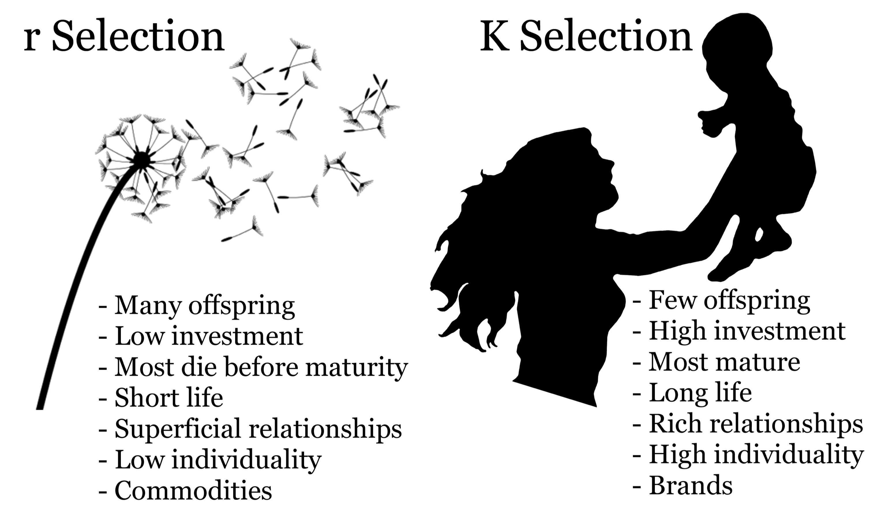
We can think of these different strategies as part of a continuum, where we will refer to the mosquito life-history strategy as an r-selected strategy, and the chimpanzee life-history strategy as a K-selected strategy. As we will discover when we begin investigating population dynamics, these terms refer to different parameters determining population growth. The parameter \(r\) describes the population growth rate, and species that have been selected to maximize population growth are likely to do so by investing less in more offspring. In contrast, the parameter K describes the point at which a given population saturates a particular environment. Species that are K-selected have attributes to maximize their competitive ability in a crowded niche.

Discussion

1. Think of examples of species that are both r- and K-selected. What is the reasoning for putting these species in a particular category?
2. Which type of species would have an advantage in a recently disturbed environment? Why?

Life history trade-offs

Every advantage has an associated cost, and the idea of life-history trade-offs underlies the diversity of life-history strategies we observe in natural environments. Let’s consider the above example where we have - on one side - an organism that invests all of its reproductive output in a single enormous brood. In fact most female mosquitoes can lie between 50-500 eggs in a single brood. On the other side we have a chimpanzee that has 3 offspring, staggered across 15 years of reproductive activity and child-rearing. We can picture these reproductive strategies by outlining their investments on a line that represents each organism’s lifetime, scaled to (0,1).

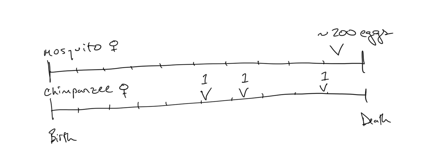
Now let’s consider what happens in-between these reproductive events… For the mosquito, it must survive its entire life before it unloads its reproductive output. If it dies before then, it achieves a lifetime fitness value \(\Phi=0\). In contrast, the chimpanzee female has staggered her reproductive output across 3 discrete events at different times throughout her life. If she dies between her first and second offspring, she still has passed her genetic material into the next generation, so has a lifetime fitness value \(\Phi > 0\). We have already defined fitness as reproduction + survival, and we can now see how both of these terms come into play when determining the lifetime fitness of an individual.

Consider again the lifetime axes of the mosquito and chimpanzee. The tick-marks represent points in time that the individual must survive (i.e. where we assess survival). The probability of mortality for the mother \(\mu\) is the probability that the female dies from one tickmark to the other. As such, the reproductive gain associated with the number of offspring listed on the lifetime axis is only obtained if the mother survives the previous periods leading up the reproduction. Let’s try to calculate the lifetime fitness of the mosquito and the chimpanzee under these very different conditions.

Let’s assume that the mother’s probability of mortality between each tickmark is the same \(\mu = 0.1\) (1%) (which by the way means that the probability of survival is \((1-\mu)\)). However, let’s assume that the probability of mortality for each individual offspring is different, capturing the tradeoff in investment. For the mosquito let’s assume the mother is capable of laying 200 eggs at the end of her life, but that the offspring mortality \(\mu_o = 0.98\) (98%). For the chimpanzee let’s assume that the mother is capable of giving birth to 3 offspring at different stages of her lifetime, and the offspring mortality is very low \(\mu_o = 0.474\) (47.4%). In other words, mosquitoes have more offspring that suffer greater mortality, and chimpanzees have fewer offspring that suffer lower mortality due to the energetic investment the mother puts into each offspring.

For the mosquito, the calculation of lifetime fitness in this context is straight forward. The mother either dies before she lays her eggs and gets \(\Phi = 0\), or dies after she lays her eggs, whereupon

where the ‘9’ represents the 9 periods it must survive prior to reproduction. (i.e. it is \((1-\mu)\) multiplied by itself 9 times)

For the chimpanzee, the calculation is more detailed. There are 4 possible outcomes here: 1) The chimp mother dies before her first offspring, such that \(\Phi = 0\); 2) The chimp mother dies between her first and second offspring; 3) The chimp mother dies between her second and third offspring; 4) The chimp mother dies after her third offspring. The lifetime fitness calculation is then

The above equation looks more complicated, but let’s break it down. First notice there are 3 separate units added together. These define the likelihood of obtaining different fitness gain associated with (from left to right): 1) reproducing once then dying, 2) reproducing twice then dying, and 3) reproducing three times then dying. This originates from the classic rule of calculating the likelihood of multiple independent or dependent events: when you are calculating the probability of events \(x\) AND \(y\) occurring, it is proportional to \({\rm prob}(x) \times {\rm prob}(y)\). When you are calculating the probability of events \(x\) OR \(y\) occurring, it is proportional to \({\rm prob}(x) + {\rm prob}(y)\).

Discussion

1. Work out what the parameters and numbers in the equation for chimp fitness represent. Use the mosquito equation to cross-reference.
2. Before you calculate anything, which strategy do you think is better?
3. Use the R web-tool below as a calculator to evaluate the lifetime fitness for both the mosquito and the chimp. Do this by entering in the above equations and plugging in the relevant values.
4. Comparing the values, discuss how such a depiction of lifetime fitness captures alternative strategies. Do you think that the differences in lifetime fitness presented here are significant?

Let’s analyze these strategies more thoroughly. Given the alternative equations for mosquito and chimpanzee fitness, let’s examine how our expectations for lifetime fitness change as a function of offspring survival \(\mu_o\).

    
    muo = seq(0,1,0.0001)

    mu_mosq = 0.1
    offspring_mosq = 200
    Phi_mosq = (1-mu_mosq)^9*((1-muo)* offspring_mosq)

    mu_chimp = 0.1
    offspring_chimp = c(1,1,1)
    Phi_chimp = (1-mu_chimp)^5*((1-muo)* offspring_chimp[1]) + (1-mu_chimp)^6*((1-muo)* sum(offspring_chimp[1:2])) + (1-mu_chimp)^8*((1-muo)* sum(offspring_chimp[1:3]))

    plot(muo,Phi_mosq,type='l',lwd=2,log='y',ylim=c(0.01,100),ylab=bquote(Lifetime~Fitness~Phi), xlab=bquote(Offspring~mortality~mu[0]))
    lines(muo,Phi_chimp,lty=2,lwd=2)

Observe that the plot shows two lines that reveal the relationship between lifetime fitness \(\Phi\) for mosquitoes (solid) and chimps (dashed) as a function of offspring mortality \(\mu_o\). Think about what these different relationships represent. Use the max() and min() to obtain the maximum and minimum value of \(\Phi_{\rm mosquito}\) and \(\Phi_{\rm chimp}\), which in the R code are denoted by Phi_mosq and Phi_chimp, respectively. Observing from the plot where the maximum and minimum values occur, how do you interpret what is being shown?

Discussion

1. Compare contrast what these relationships tell you about the relative fitness of mosquitoes vs. chimpanzees when \(\mu_o\) is small vs. large.
2. How do you interpret the y-axis?
3. The values for \(\mu_o\) provided above point to a particular coordinate on the \(\Phi_{\rm mosquito}\) and \(\Phi_{\rm chimp}\) lines on the plot. Interpret what this tells us about the mosquito and chimp life history strategies.

Decision-making and future fitness

Above we explored how to assess the accumulated fitness consequences of alternative strategies spanning the r-K selection gradient, but where these strategies are static. Of course, individual behaviors are dynamic in response to real-time conditions, and do not generally have static strategies. In other words, individuals within species react to external conditions by changing their behavior and the cumulation of these reactions have a large impact on – and often define – their life-history strategies.

We can imagine a species’ behavior as a set of iterative yes/no decisions. Now don’t make the mistake and read decision as a cognitive choice… the decisions that species make characterizing their behaviors are selected for over evolutionary time, and thus are encoded in their genes, but do not always mean that they are cognitively thinking through and weighing the costs/benefits of particular decisions. For example, when a reed warbler decides whether or not to forage once more to gather an extra amount of food for her chicks before the sun sets for the night, the decision need not be a cognitive calculation, but a behavioral predisposition fueled by her genes that make her more or less likely to decide one way or the other. Linking these binary yes/no decisions to the above activity, after sexual maturity both chimps and mosquitoes make decisions whether or not to invest in reproduction throughout their lives… the mosquito decision tree pertaining to the above example is then: (no no no no no no no no no yes), and the chimp decision tree is (no no no no no yes yes no no yes). So, in this context, these genetically-determined ‘decisions’ make the strategy.

We will assume that natural selection over evolutionary time has resulted in species with behaviors the maximize their lifetime fitness. We will assume this in the context of a yes/no decision. Let’s use the example of a warbler deciding whether or not to gather one additional morsel of food for her brood before the sun sets for the day, which is a binary yes/no decision.

Some definitions:

• \(\Phi\) = The value of future reproductive success
• \(\phi\) = The amount of \(\Phi\) that is at stake in this decision
• \(a\) = the proportionate increase in \(\phi\) that would result if there is a positive (yes) response
• \(c\) = the cost of \(a\)
• \(b\) = the proportionate decrease in \(\phi\) if there is a negative (no)

YES Decision In words, we want to assess what \(\Phi\) will be on the other side of this yes/no decision. If the decision is a yes, we will gain something but at a cost. The amount \(\phi\) is at stake, and a positive response will recover a proportionate amount of \(\phi\) given by \(a\) at cost \(c\). We will call this modified fitness \(\Phi^\prime\). Both \(a\) and \(c\) vary between 0 and 1. Use the extreme values of 0 and 1 for \(a\) and \(c\) to understand how they impact lifetime fitness assuming a Yes decision. I recommend first setting \(c=0\) and examining the cases where \(a=0\) (what does this mean?) and \(a=1\) (what does this mean?).

NO Decision If the decision is a no, the modified fitness is \(\Phi^{\prime \prime}\) we will assume that we lose what is at stake, proportional to \(b\). So if \(b=1\), all of what is at stake (all of \(\phi\)) is lost; if \(b=0\), none of what is at stake is lost.

So the question now is… when will selection favor the positive response (resulting in \(\Phi^\prime\)) and when will it favor the negative response (resulting in \(\Phi^{\prime \prime}\))? Based on our assumption that the process of evolution selects for the fitness-maximizing strategy, we can see that the positive response will be favored if \(\Phi^\prime > \Phi^{\prime \prime}\) and the negative response will be favored if \(\Phi^\prime < \Phi^{\prime \prime}\).

Let us now explore these relationships graphically. We will first set values for the different parameters in the above model, and examine how \(\Phi^\prime\) and \(\Phi^{\prime\prime}\) vary as a function of an increasing amount of fitness at stake \(\phi\) (i.e. we will examine \(\Phi^\prime\) and \(\Phi^{\prime\prime}\) as a function of \(\phi\)). In other words, how does the lifetime fitness following a positive vs. negative response change as the stakes \(\phi\) increase?

    # First set the total amount of lifetime fitness before the yes/no decision
    Phi = 100
    # We are looking at how the fitness consequences of a yes/no decision 
    # change with increasing stakes, so this needs to be a vector that starts 
    # at 0 (no stakes) and ends at Phi (all is at stake)
    phi = seq(0,100,1)

    # We will set the proportionate gain in phi to be 0.5
    a = 0.5

    # And we will specify that the loss in phi if the decision 
    # is negative is (1/2)a
    b = (1/2)*a

    #For now we will ignore the cost
    c = 0.0

    #Calculate Phi following a yes response
    Phi_prime = (1+a)*phi + (1-c)*(Phi-phi)

    #Calculate Phi following a no response
    Phi_2prime = (1-b)*phi + (Phi - phi)

    #Plot Phi^prime as a BLUE line
    plot(phi,Phi_prime,type='l',col='blue',xlab='Part of Phi at stake',ylab='Response',ylim=c(50,150))
    #Plot Phi^primeprime as a RED line
    lines(phi,Phi_2prime,col='red')

    # We will now add in a cost to see how that changes the relationships
    # Will we change c to 0.25, and then recalculate Phi^prime
    c = 0.25
    # Let's add the new Phi^prime as a DASHED blue line
    Phi_prime = (1+a)*phi + (1-c)*(Phi-phi)
    lines(phi,Phi_prime,col='blue',lty = 2)

Discussion

1. Looking only at the SOLID blue \(\Phi^\prime\) and SOLID red \(\Phi^{\prime\prime}\) lines, what do we observe? Remember that in this case the gain of a positive response is always greater than the loss of a negative response, and there is no cost associated with the gain.
2. When is \(\Phi^\prime > \Phi^{\prime\prime}\)?
3. Now consider the case when \(c=0.25\). So we are comparing the DASHED blue \(\Phi^\prime\) line to the SOLID red \(\Phi^{\prime\prime}\) line. What do you observe?
4. When is \(\Phi^\prime > \Phi^{\prime\prime}\), and when is it not? Does this make sense given the difference in cost from the solid to dashed blue line?
5. Imagine these two different scenarios… where would these cases fall on the above graph, all other things being equal? A mother reed warbler is deciding whether or not to forage once more before retiring for the night….
   • in case 1, her offspring are near starvation
   • in case 2, her offspring are fat and healthy